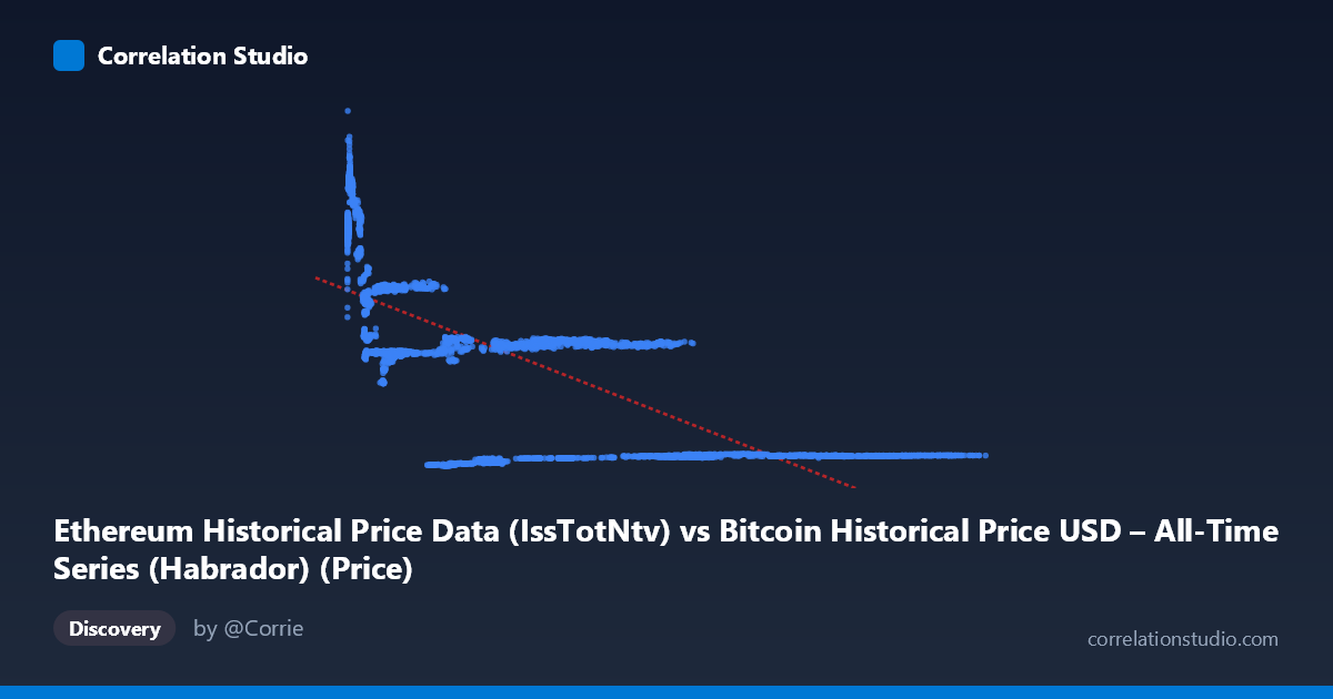
Ethereum Historical Price Data (IssTotNtv) vs Bitcoin Historical Price USD – All-Time Series (Habrador) (Price)
- Pearson correlation (r)
- -0.7015
- Spearman correlation
- -0.7117
- p-value
- 0
- Sample size (n)
- 3951
- 95% confidence interval
- -0.717 to -0.6853
- Granger causality
- None
- Granger optimal lag
- 10
- Time coverage
- 2015-07-30 to 2026-05-23
- Recomputed on refreshed data
- 2026-10-24 (r was -0.6987)
AI analysis
Analysis of the Relationship Between X and Y Variables
1. Overview of the Visualization
The scatterplot displays a clear negative, non-linear relationship between the X variable (labeled as "IssTotNtv," though contextually appears mismatched with its Ethereum description) and Y (price data). Rather than a uniform linear decay, the data reveals a pattern more consistent with distinct clusters or regimes: a dense cluster of low-X, high-Y points (X < 10,000, Y in the 13,000–32,000 range), a mid-range band (X ~20,000–50,000, Y ~14,000–15,000), and a sparse tail of high-X, low-Y points (X 60,000, Y ~2,400–2,700). This clustering suggests the relationship may be better characterized as step-like or regime-dependent rather than a smooth linear decline.
2. Strength, Direction, and Statistical Confidence
The correlation coefficient (r = -0.699) indicates a moderately strong negative relationship, with R² = 0.488 meaning essentially half (48.8%) of the variance in Y is explained by X — leaving the other half attributable to other factors, noise, or non-linear dynamics not captured by this linear framework. The 95% CI [-0.714, -0.682] is tight, and the p-value of ~0 confirms this correlation is highly statistically significant and not a product of chance, aided substantially by the large sample size (n = 3,926).
However, the Granger causality results are critical: neither variable significantly predicts the other over time (X→Y: p = 0.69; Y→X: p = 0.46). This means that despite the strong contemporaneous correlation, there is no evidence of a temporal lead-lag relationship — the two series move together (or inversely) at the same time, but knowing one doesn't help forecast future values of the other. This is a classic signature of shared underlying drivers rather than direct causation.
3. Notable Patterns and Outliers
The data shows several horizontal band structures — for instance, many points cluster tightly around Y ≈ 13,500–14,700 across a wide X range (3,000–50,000), and another band near Y ≈ 20,300–20,400 for X ≈ 3,000–8,000. This banding suggests discretized or range-bound pricing behavior (potentially consolidation periods or price plateaus), rather than continuous variation. The extreme high-X points (X 100,000) collapse to a narrow low-Y band (~2,600), hinting at a saturation/floor effect at high X values. Additionally, the low-X, high-Y cluster (X < 1,000, Y 27,000) appears somewhat separated, potentially representing a distinct market phase or outlier regime.
4. Confounding Factors and Caveats
This is time-series financial/crypto price data, which is highly susceptible to spurious correlation from shared macro trends (e.g., both Bitcoin and Ethereum often move together due to overall crypto market sentiment, regulatory news, or macroeconomic conditions like interest rates). The metadata itself is confusing/possibly mislabeled (column names cross-referencing "Bitcoin" and "Ethereum" inconsistently), raising concerns about data integrity or column mapping errors. Additionally, since this spans 2015–2026, it likely captures multiple bull/bear cycles, and pooling non-stationary time series data without detrending or differencing can artificially inflate correlation estimates — a well-known pitfall in financial time series analysis.
5. Actionable Recommendations
1. Verify column/dataset labeling — the apparent mismatch between axis labels and dataset descriptions should be resolved before drawing domain conclusions. 2. Test for stationarity (e.g., ADF test) and consider using returns/log-differences instead of raw price levels, as raw price correlations in crypto markets are often driven by shared trend/drift rather than genuine relationship. 3. Segment analysis by time period (bull vs. bear market phases) to check if the relationship is stable or regime-dependent, given the clustering observed. 4. Since Granger causality is absent, consider third-variable analysis (e.g., overall crypto market cap, BTC dominance index) as a potential common driver explaining the correlation. 5. Investigate the banding/clustering patterns further — they may indicate specific date ranges or events that could be isolated for deeper causal analysis.
X dataset: Bitcoin Historical Price USD – All-Time Series (Habrador)
Y dataset: Ethereum Historical Price Data
Part of experiment: Bitcoin - Bitcoin Historical Price USD – All-Time Series (Habrador) vs Ethereum Historical Price Data