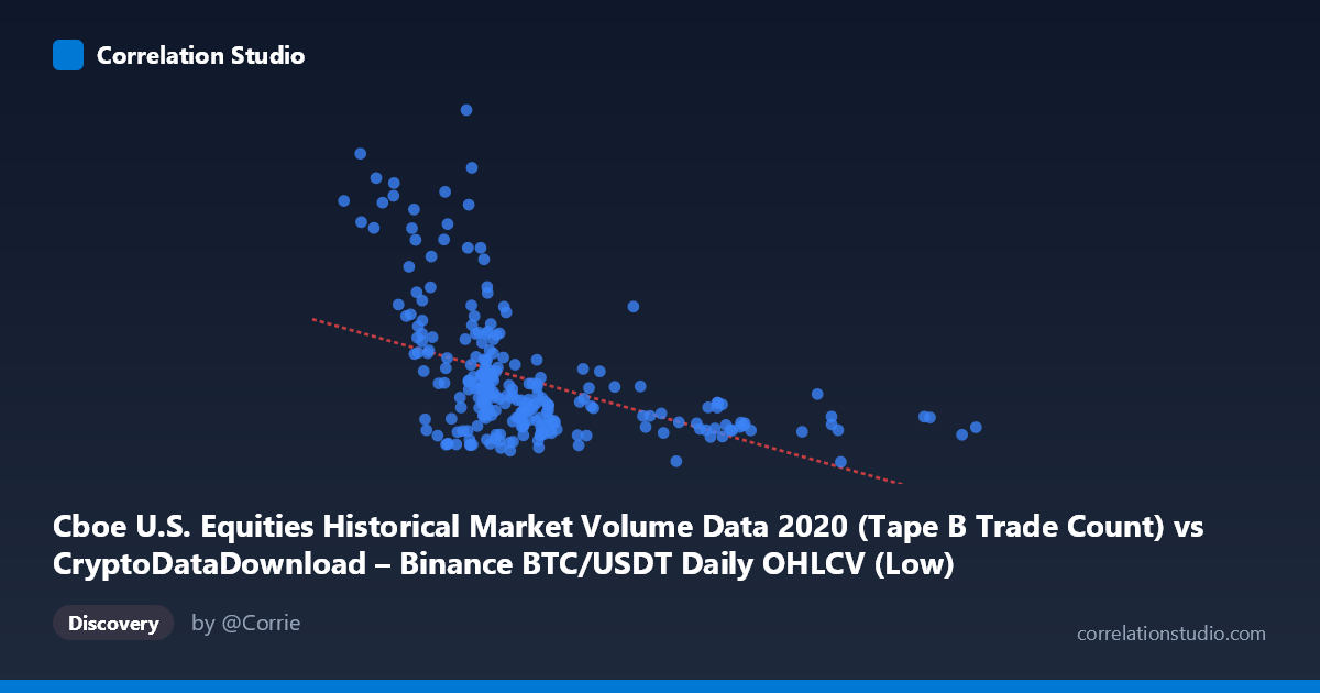
Cboe U.S. Equities Historical Market Volume Data 2020 (Tape B Trade Count) vs CryptoDataDownload – Binance BTC/USDT Daily OHLCV (Low)
- Pearson correlation (r)
- -0.4698
- Spearman correlation
- -0.5555
- p-value
- 0
- Sample size (n)
- 253
- 95% confidence interval
- -0.5606 to -0.3677
- Granger causality
- None
- Granger optimal lag
- 10
- Time coverage
- 2020-01-02 to 2020-12-31
AI analysis
Analysis: Cboe Trade Count vs. BTC/USDT Low Price (2020)
1. What the Visualization Reveals
The scatterplot shows a modest negative relationship between Cboe Tape B trade counts and BTC/USDT daily low prices. Most points cluster in a dense region where trade counts fall between roughly 7,000–12,000 and Y-values sit between $200,000–$600,000 (note: despite the column label "Low," these values are far above typical BTC price ranges for 2020, suggesting a scaling/unit anomaly worth investigating — see caveats below). Beyond this core cluster, a sparser tail extends to higher X-values (17,000–28,000) where Y-values compress into a narrower, lower band (~$250,000–$350,000), contributing most of the visible downward slope.
2. Strength, Direction, and Statistical Confidence
The correlation coefficient (r = -0.470) indicates a moderate negative linear relationship, but R² = 0.221 means only about 22% of the variance in Y is explained by X — leaving nearly 80% attributable to other factors or noise. The 95% CI [-0.561, -0.368] is reasonably tight and excludes zero, and the p-value (2.67E-15) confirms this correlation is highly statistically significant and not due to chance, given n=253. However, statistical significance ≠ practical strength — the relationship, while real, is weak-to-moderate and would have limited standalone predictive power.
Critically, the Granger causality tests show no significant temporal predictive direction in either direction (X→Y: p=0.746; Y→X: p=0.132). This suggests the contemporaneous correlation is not driven by one series leading the other in time — it may instead reflect a shared external driver, coincidental trending, or a spurious relationship arising from both series' independent time-based patterns during 2020.
3. Notable Patterns and Outliers
Several outliers stand out sharply: (8445, 1,222,154), (3782, 950,884), (8531, 939,285), and (5688, 1,003,994) — all with unusually high Y-values relative to their X position, sitting far above the main cluster. These points likely correspond to specific dates with anomalous market activity (possibly March 2020 COVID crash volatility or other 2020 disruptions) and exert outsized leverage on the regression line, given their extreme Y-values combined with low-to-mid X-values. Additionally, the low-X tail (X < 6,000) is sparse and dominated by these high-Y outliers, meaning the left edge of the fitted line is poorly constrained by data density.
4. Confounding Factors and Caveats
This pairing is unusual: it combines U.S. equities market trade counts (Cboe Tape B) with a cryptocurrency price series (BTC/USDT), two structurally different markets. Any correlation is likely driven by shared macro conditions in 2020 — notably the COVID-19 crash and subsequent recovery, which simultaneously affected equity trading volumes and crypto prices — rather than a direct mechanistic link. Both series are also time-ordered (daily, 2020), making them subject to autocorrelation and trending, which can inflate correlation estimates between otherwise unrelated series (a classic spurious-correlation risk with non-stationary time series). The label "Low" for BTC/USDT seems inconsistent with actual 2020 BTC price ranges (which topped out near $29,000), suggesting the Y-axis values may be misaligned, scaled, or mislabeled — this should be verified before drawing economic conclusions.
5. Recommendations for Further Investigation
1. Verify data integrity: confirm the Y-axis units/scaling and check whether "Low" values genuinely correspond to BTC price or were mis-joined with another metric. 2. Detrend and test stationarity: apply differencing or use returns instead of levels for both series, then re-run correlation/Granger tests to rule out spurious time-trend correlation. 3. Control for macro confounders: introduce a third variable (e.g., VIX, overall market volume, or a COVID-timeline indicator) to test whether the relationship survives after controlling for shared crisis-period dynamics. 4. Robustness check on outliers: re-run the regression after excluding the four high-leverage outlier points to assess sensitivity of r² and the slope estimate. 5. Given the lack of Granger causality, avoid using this pair for predictive/trading models; treat the correlation as descriptive/contextual only, not causal or forecastable.
X dataset: CryptoDataDownload – Binance BTC/USDT Daily OHLCV
Y dataset: Cboe U.S. Equities Historical Market Volume Data 2020
Part of experiment: Bitcoin - CryptoDataDownload – Binance BTC/USDT Daily OHLCV vs Cboe U.S. Equities Historical Market Volume Data 2020