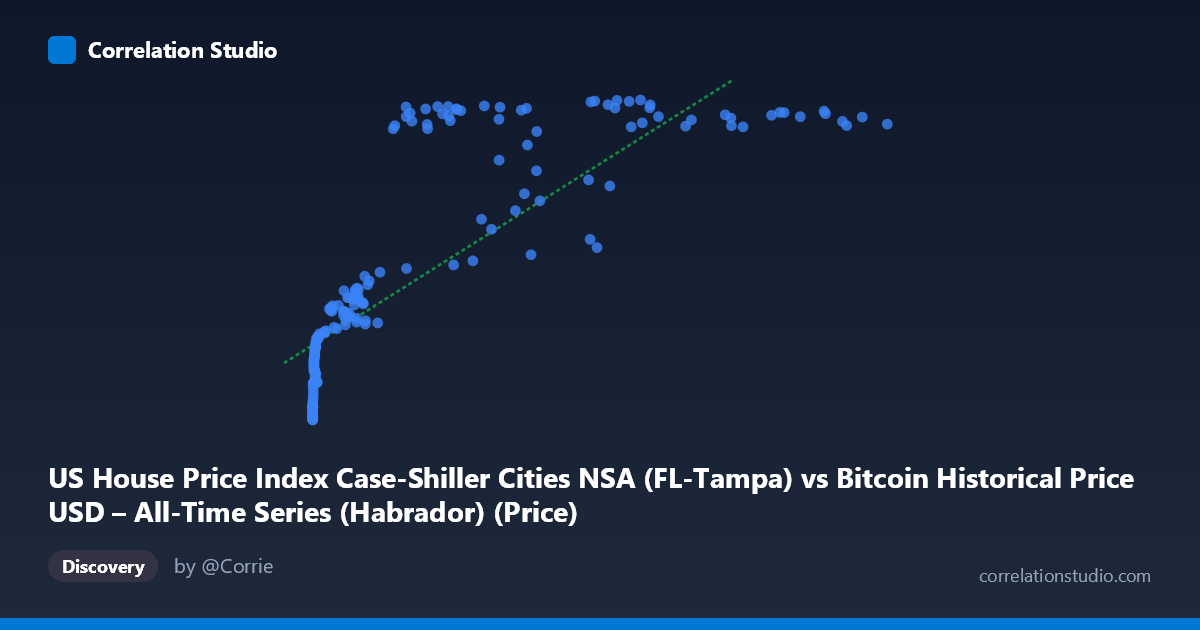
US House Price Index Case-Shiller Cities NSA (FL-Tampa) vs Bitcoin Historical Price USD – All-Time Series (Habrador) (Price)
- Pearson correlation (r)
- 0.8055
- Spearman correlation
- 0.9479
- p-value
- 0
- Sample size (n)
- 187
- 95% confidence interval
- 0.7485 to 0.8507
- Granger causality
- None
- Granger optimal lag
- 9
AI analysis
Analysis: Bitcoin Price vs. Tampa Case-Shiller Home Price Index
1. What the Visualization Reveals
The scatterplot shows a strongly positive but distinctly non-linear relationship between Bitcoin's historical USD price and the Tampa Case-Shiller Home Price Index. At low Bitcoin values (near $0–$1,000), the housing index is compressed in a narrow band (roughly 125–200), rising slowly. As Bitcoin climbs into the tens of thousands, the index rises more steeply before appearing to plateau/saturate in the mid-to-high 300s at the largest Bitcoin values (even dipping slightly at the very top, e.g., ~118,670 → 368.25 vs. ~58,254 → 387.26). This curved, saturating shape is characteristic of a logarithmic or power relationship rather than a straight line.
2. Strength, Direction, and Uncertainty
The Pearson correlation (r = 0.8055, r² = 0.6488) indicates a strong positive linear association, with the linear model explaining about 65% of the variance in the housing index — leaving roughly 35% unexplained. The 95% CI [0.7485, 0.8507] is tight and does not cross zero, and the p-value is effectively 0, so the correlation is highly statistically significant and not a chance artifact of this sample. However, statistical significance here reflects the strength of co-movement over time, not necessarily a causal or economically meaningful link. Critically, Granger causality tests show no predictive direction in either direction (Bitcoin→Housing: p=0.59; Housing→Bitcoin: p=0.79). This means neither series' past values help forecast the other's future values — the correlation is likely driven by both series independently trending upward over the same calendar period (2010–2026), not by one variable influencing the other.
3. Notable Patterns and Outliers
Several features stand out: - Compression at low X: Hundreds of points with Bitcoin < $1,000 map to a tight Y-range (125–200), consistent with Bitcoin's early years (2010–2013) coinciding with a slowly recovering post-2008 housing market. - Divergence/plateau at high X: Above ~$40,000–50,000 Bitcoin price, Y values cluster in the 350–390 range with high scatter (e.g., $41,869→296.77 vs. $44,354→350.99), suggesting the housing index has structurally saturated while Bitcoin continues to swing wildly (its known boom-bust cycles). - Non-monotonic dips: Points like $45,092→260.34 and $56,973→322.17 amid neighboring higher-Y points at similar X suggest Bitcoin's volatility (bear market crashes) doesn't track the smoother, mostly monotonic housing index. - The note that Spearman ρ likely exceeds Pearson r confirms the visual: a log-transform of X would likely straighten the relationship and improve fit.
4. Confounding Factors and Caveats
This is a classic case of spurious correlation via shared time trend. Both Bitcoin prices and US home prices have risen substantially over 2010–2026 due to largely unrelated macro forces: Bitcoin's adoption/speculation cycles vs. housing driven by low interest rates, supply constraints, and regional Tampa market dynamics (post-pandemic migration, etc.). Any two upward-trending time series will show inflated correlation without genuine causal linkage. Additional confounders include broad monetary policy (QE, low rates 2010–2021, inflation post-2021) that could simultaneously push both asset classes higher, and the mismatched volatility/liquidity profiles of the two assets (Bitcoin is far more volatile and mean-reverting within cycles than housing).
5. Actionable Insights
- Detrend before concluding causality: Analyze returns/percent changes or first-differenced series rather than levels, and re-run correlation and Granger tests — the relationship will likely weaken substantially once the shared trend is removed. - Try a log-linear model: Given the saturating curve and the Spearman/Pearson discrepancy, fit y = a·ln(x) + b or a power-law model to better capture the relationship and compare R². - Treat as coincidental co-trending, not predictive: Given the null Granger results, this correlation should not be used for trading or forecasting one asset from the other; it's more a statistical artifact of the sample period than an economic signal. - Segment by market regime: Compare correlation within Bitcoin bull vs. bear phases to see if the relationship holds or disappears — this would clarify whether the correlation is genuinely structural or purely an artifact of both series rising over a 15-year window.
X dataset: Bitcoin Historical Price USD – All-Time Series (Habrador)
Y dataset: US House Price Index Case-Shiller Cities NSA
Part of experiment: Bitcoin - Bitcoin Historical Price USD – All-Time Series (Habrador) vs US House Price Index Case-Shiller Cities NSA