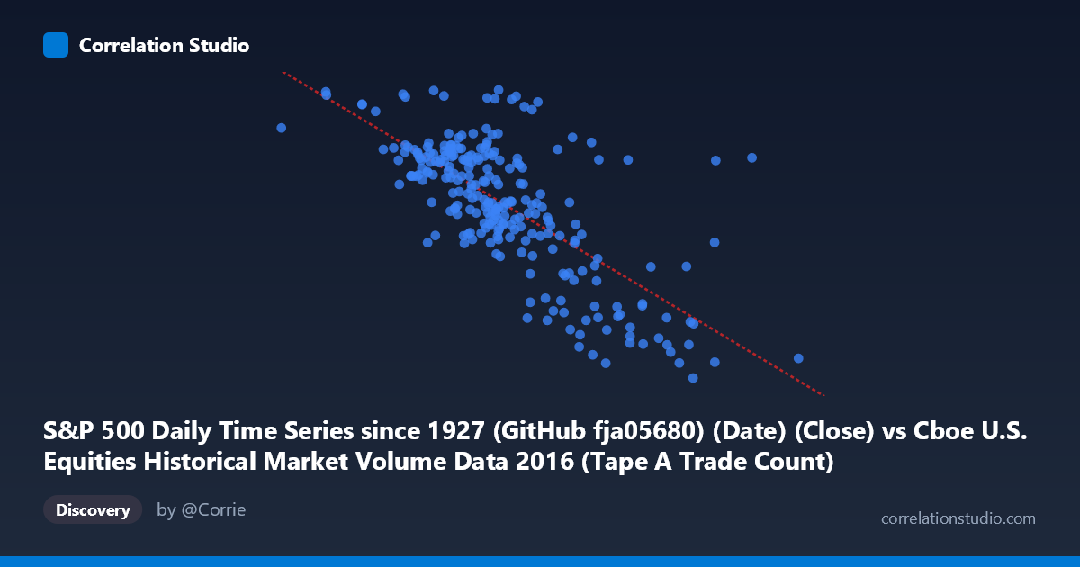
S&P 500 Daily Time Series since 1927 (GitHub fja05680) (Date) (Close) vs Cboe U.S. Equities Historical Market Volume Data 2016 (Tape A Trade Count)

Pearson correlation (r): -0.7131
Spearman correlation: -0.6644
p-value: 0
Sample size (n): 252
95% confidence interval: -0.7689 to -0.6465
Granger causality: None
Granger optimal lag: 4
Time coverage: 2016-01-04 to 2016-12-30

AI analysis

Analysis: S&P 500 Close Price vs. Cboe Tape A Trade Count (2016)

Relationship Overview The scatterplot reveals a moderately strong negative relationship between the S&P 500 closing price (X-axis) and Cboe Tape A Trade Count (Y-axis) across 252 trading days in 2016. As the index climbed from roughly 1,829 to 2,272, trade counts generally declined — suggesting that calmer, trending bull-market conditions in 2016 were associated with reduced transactional activity on Tape A venues. The linear regression (y = −0.00024334x + 2,432.63) captures this inverse slope cleanly, with the cloud of points showing a discernible downward sweep from left (lower prices, higher counts) to right (higher prices, lower counts).

Correlation Strength and Statistical Interpretation The Pearson correlation of r = −0.713 indicates a moderately strong negative association, and the R² of 0.509 means that approximately 50.9% of the variance in Tape A trade counts is statistically explained by the S&P 500 closing level. That is a practically meaningful share, but it equally implies that ~49% of variance lies elsewhere. The 95% confidence interval of [−0.769, −0.647] is notably tight and does not cross zero, and the p-value is effectively 0 across a population of N = 3,622 — so the correlation is highly unlikely to be a sampling artifact. However, the Granger causality tests tell a more cautious story: neither direction (X→Y nor Y→X) reaches significance at a 4-period lag (F ≈ 0.30, p = 0.88 for X→Y; F ≈ 0.62, p = 0.65 for Y→X). This means that while a strong contemporaneous correlation exists, neither variable reliably predicts the other's future values in this sample. Correlation here reflects co-movement with a common driver, not a lead-lag predictive mechanism.

Patterns, Clusters, and Outliers The data separates into two loose behavioral zones. A left-side cluster (S&P 500 roughly 900–1,400) shows higher and more dispersed trade counts, broadly consistent with early-2016 volatility and the market correction in January–February. A right-side cluster (1,400–1,900+) shows compressed trade counts congregating near 1,870–2,100, reflecting the steadier post-recovery climb. Several notable outliers are visible: one point near (1,000, 2,265) sits well above the regression line, suggesting an anomalously high trade-count day at a relatively low price level — possibly a volatility event. Conversely, a handful of points in the upper-right (~1,860–2,013, trade counts near 1,870–1,940) fall below the trend, representing unusually quiet sessions at elevated price levels. The scatter also shows modest heteroscedasticity: variance in trade counts is wider at lower price levels and narrows as prices rise, which can slightly inflate the apparent fit of a linear model.

Confounding Factors and Caveats Several important confounds complicate direct interpretation. Seasonality is a primary concern — 2016 began with a sharp selloff and ended with a post-election rally, meaning both price level and trading activity were simultaneously driven by macro events (China slowdown fears, Brexit, U.S. election) rather than one causing the other. Secular fragmentation in equity markets means Tape A volume is only one slice of total trading; routing behavior to dark pools or other tapes could independently shift Tape A counts regardless of price. The unit mismatch is also worth flagging: X is an index level (not a return), so the correlation partly reflects the time-series trend rather than a true economic mechanism. Using index returns or volatility (e.g., VIX) instead of price levels would yield a more structurally meaningful test. Finally, 252 paired samples from a single calendar year limits generalizability.

Actionable Insights and Further Investigation The absence of Granger causality despite a strong contemporaneous correlation points toward a shared latent driver — most likely realized volatility or investor uncertainty — as the more fundamental variable worth modeling. Recommended next steps include: (1) Replace S&P 500 close with VIX or realized volatility to test whether the volume relationship is actually mediated by fear/uncertainty rather than price level per se; (2) Decompose Tape A counts by trade size to distinguish retail from institutional behavior across the price range; (3) Extend the analysis to multiple years to determine whether 2016's specific macro arc (sell-off → recovery → election rally) is driving the pattern or whether it persists structurally; and (4) Apply a regime-switching or piecewise regression given the visual evidence of two distinct behavioral clusters, which may outperform the single linear fit indicated by the modest R² of ~0.51.

X dataset: Cboe U.S. Equities Historical Market Volume Data 2016

Y dataset: S&P 500 Daily Time Series since 1927 (GitHub fja05680) (Date)

Part of experiment: Daily - Cboe U.S. Equities Historical Market Volume Data 2016 vs S&P 500 Daily Time Series since 1927 (GitHub fja05680) (Date)