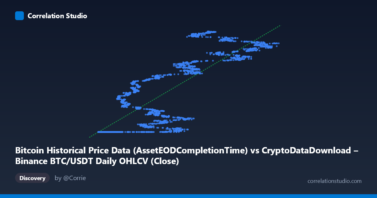
Bitcoin Historical Price Data (AssetEODCompletionTime) vs CryptoDataDownload – Binance BTC/USDT Daily OHLCV (Close)

Pearson correlation (r): 0.8518
Spearman correlation: 0.8876
p-value: 0
Sample size (n): 3191
95% confidence interval: 0.842 to 0.861
Granger causality: None
Granger optimal lag: 10

AI analysis

Analysis: BTC/USDT Completion Time vs. Close Price

1. What the Visualization Reveals

This scatterplot is unusual in that it's not comparing two independent economic variables — it's plotting a timestamp-derived column ("AssetEODCompletionTime") against the corresponding daily closing price of the same BTC/USDT dataset. Effectively, the X-axis is a proxy for time or sequence order, and the Y-axis is the price series itself. The data reveals a distinctive pattern: a dense horizontal cluster at low X-values (~3,000–25,000) where Y sits tightly near $1.614B, followed by a steep, more scattered climb as X increases toward the 80,000–125,000 range, where Y reaches $1.73B–$1.78B. This is characteristic of a price series that was flat/consolidating early on and then trended upward with increasing volatility.

2. Strength, Direction, and Uncertainty

The correlation is strong and positive (r = 0.852, r² = 0.726), meaning roughly 73% of the variance in Y is statistically explained by X — a substantial but not complete relationship, leaving over a quarter of variance driven by other factors (likely short-term volatility, market microstructure, or noise not captured by this linear fit). The confidence interval [0.842, 0.861] is tight, and the p-value of ~0 confirms this correlation is not due to chance at this sample size (n=3,191). However, correlation strength should not be conflated with causal or predictive power: the Granger causality tests show no significant predictive direction in either direction (X→Y: p=0.326; Y→X: p=0.168). This means that despite the strong contemporaneous linear association, neither variable helps forecast future values of the other beyond what each series' own history provides — an important distinction, especially since X appears to be a time/order proxy rather than an independent market variable.

3. Notable Patterns and Non-linear Features

The relationship is clearly not linear — it resembles a hockey-stick or piecewise structure. There's a large plateau where Y is essentially constant (~$1.614B) across a wide range of low X values, suggesting either a data artifact (repeated/padded timestamps) or a genuine early flat-price regime. Beyond this plateau, Y increases with increasing dispersion/variance at higher X, producing a fan-like spread. This heteroskedasticity (variance increasing with X) violates a core assumption of simple linear regression, meaning the r²=0.726 statistic may overstate the "goodness" of a single linear model across the full range — a segmented or non-linear (e.g., logarithmic, piecewise) model would likely fit much better.

4. Confounding Factors and Caveats

Several caveats are critical here: - X is likely a timestamp/sequence variable, not an independent economic driver — so this is closer to a time-series trend analysis than a true bivariate correlation between two market fundamentals. - The flat cluster at low X with identical Y values (1,614,337,xxx) strongly suggests repeated or forward-filled values, possibly from missing data being backfilled with a constant, which would artificially inflate correlation. - Autocorrelation in both time-ordered series violates independence assumptions underlying the p-value calculation, meaning statistical significance may be overstated (effective sample size is likely much smaller than n=3,191). - Bitcoin's known volatility clustering and regime-dependent behavior (bull/bear cycles) means a single global linear/correlation statistic obscures very different local dynamics.

5. Actionable Insights

- Investigate the flat plateau: confirm whether the repeated Y-values at low X reflect real market conditions (e.g., exchange downtime, early illiquid trading) or a data-quality/padding issue — this could materially change the correlation once cleaned. - Re-run analysis on log(Y) or with a piecewise/segmented regression to better capture the non-linear, heteroskedastic structure. - Clarify the true nature of the X variable — if it's a timestamp, standard time-series techniques (trend decomposition, ARIMA, changepoint detection) are more appropriate than correlation/regression. - Given the null Granger causality result, avoid using this relationship for predictive/forecasting purposes; the strong r² reflects shared trend, not directional forecasting power.

X dataset: CryptoDataDownload – Binance BTC/USDT Daily OHLCV

Y dataset: Bitcoin Historical Price Data

Part of experiment: Bitcoin - CryptoDataDownload – Binance BTC/USDT Daily OHLCV vs Bitcoin Historical Price Data