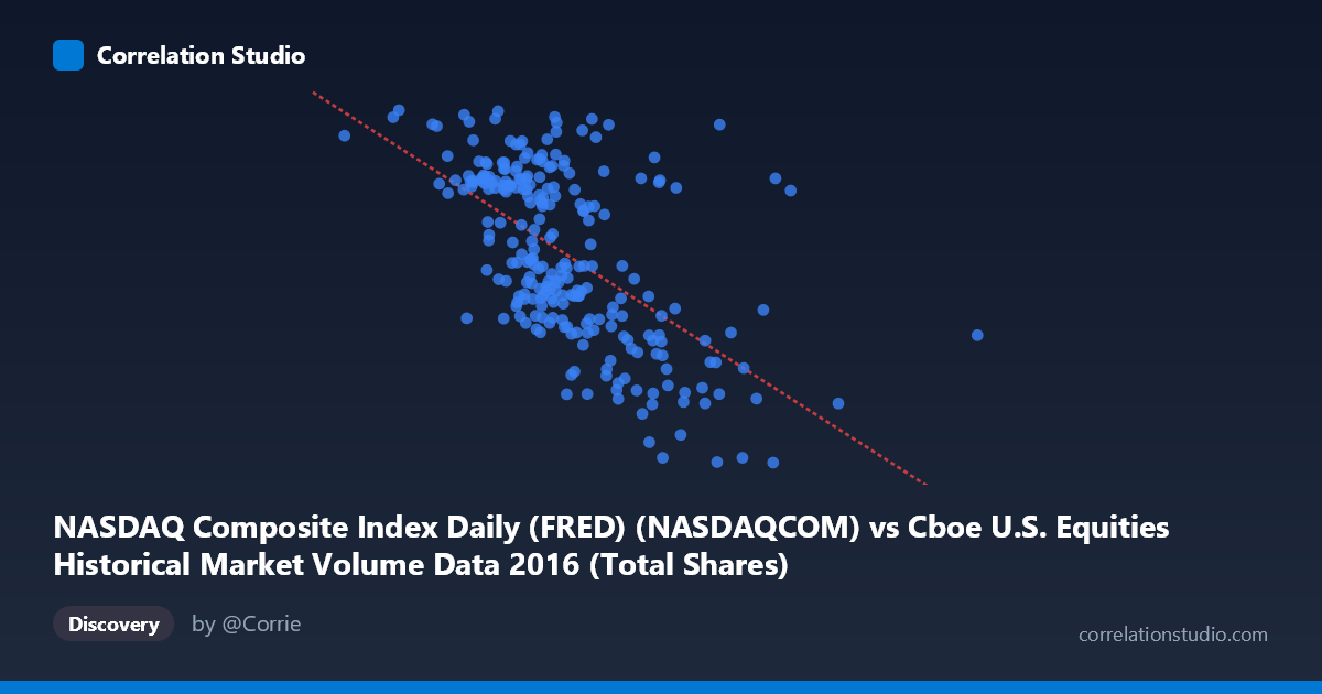
NASDAQ Composite Index Daily (FRED) (NASDAQCOM) vs Cboe U.S. Equities Historical Market Volume Data 2016 (Total Shares)
- Pearson correlation (r)
- -0.5916
- Spearman correlation
- -0.6064
- p-value
- 0
- Sample size (n)
- 252
- 95% confidence interval
- -0.6665 to -0.505
- Granger causality
- None
- Granger optimal lag
- 10
AI analysis
Analysis: NASDAQ Composite Index vs. U.S. Equities Market Volume (2016)
Relationship Overview
The scatterplot reveals a moderate negative relationship between the NASDAQ Composite Index daily closing value (X) and total shares traded across U.S. equities exchanges (Y). As the NASDAQ index climbed higher throughout 2016, total share volume tended to decline — a pattern that is visually apparent in the downward-sloping regression line (y = -1.574×10⁻⁶x + 5794.8). This inverse relationship is consistent with a well-documented market phenomenon: rising, trending markets tend to generate less urgency-driven trading activity, while lower index levels are often associated with volatility events that spike participation and share turnover. The data spans the full 2016 calendar year, capturing a range of market conditions from early-year turbulence to the post-election rally in Q4.
Correlation Strength and Statistical Significance
The Pearson correlation of r = -0.5916 indicates a moderate-to-strong negative association, and the R² of 0.35 means that approximately 35% of the variance in total shares traded is explained by the NASDAQ index level — a meaningful but incomplete explanatory picture, leaving 65% of variance attributable to other factors. The 95% confidence interval of [-0.6665, -0.5050] is entirely negative and does not include zero, reinforcing that the direction of the relationship is robust. The p-value of essentially 0 (against a population of N = 3,622) confirms this is not a chance finding. However, the Granger causality results tell a more cautionary story: neither direction (X→Y nor Y→X) reaches significance (F = 0.31, p = 0.98 and F = 0.65, p = 0.77 respectively at optimal lag 10). This means that while the two series are correlated contemporaneously, neither variable reliably predicts the other in a temporal, lead-lag sense — the relationship reflects co-movement rather than a directional causal mechanism.
Notable Patterns, Clusters, and Outliers
Several structural features stand out in the sample points. There is a visible cluster of high-volume observations (Y 5,200 shares) concentrated at lower NASDAQ index levels (roughly X < 470M), consistent with the early-2016 selloff period when volatility was elevated. Conversely, the highest index values (X 630M–700M+) are paired with notably low share volumes (Y ≈ 4,450–4,510), pointing to the quieter, lower-turnover conditions of the late-year rally. A few points — such as (369,051,288; 5,471) and (549,126,514; 5,457) — appear as potential outliers that deviate from the regression line, suggesting episodic high-volume days that may correspond to index rebalancing events, option expiration dates, or macro announcements rather than index-level effects. The spread of residuals also appears to widen at mid-range X values, hinting at possible heteroscedasticity in the relationship.
Confounding Factors and Caveats
Several important caveats limit a straightforward causal interpretation. First, 2016 was an unusual year with distinct volatility regimes — the January-February global selloff, the Brexit shock in June, and the post-U.S. election surge in November/December — meaning the negative correlation may partly reflect these discrete macro episodes rather than a stable structural relationship. Second, share volume is influenced by many factors independent of index level, including algorithmic trading activity, ETF rebalancing, corporate actions, and options expiration cycles, all of which can decouple volume from price trends. Third, the datasets have different conceptual origins (Cboe exchange volume vs. NASDAQ index), and any compositional changes in listed securities or exchange market share during 2016 could introduce noise. Finally, the unit mismatch between an index value and total shares traded means the regression coefficient (-1.57×10⁻⁶) has limited intuitive interpretability without further normalization.
Actionable Insights and Further Investigation
Practitioners interested in this relationship should consider several next steps. Segmenting by market regime (e.g., low-VIX vs. high-VIX periods, or pre/post-Brexit) would help determine whether the negative correlation holds consistently or is driven by a handful of turbulent episodes. Incorporating implied volatility (VIX) as a third variable could reveal whether it serves as a common driver of both lower index levels and higher volumes, potentially explaining much of the residual variance. It would also be valuable to test this correlation across multiple years to assess whether 2016 is representative or anomalous. Given the absence of Granger causality, strategies that attempt to use one variable to predict the other in trading contexts should be treated with skepticism; any signal here appears contemporaneous rather than predictive. Finally, exploring whether non-linear models (e.g., piecewise regression or LOWESS smoothing) improve fit could reveal threshold effects around critical index levels.
X dataset: Cboe U.S. Equities Historical Market Volume Data 2016
Y dataset: NASDAQ Composite Index Daily (FRED)
Part of experiment: Daily - Cboe U.S. Equities Historical Market Volume Data 2016 vs NASDAQ Composite Index Daily (FRED)