Datahub.io – WTI Daily Spot Price CSV (Price) vs Cboe U.S. Equities Historical Market Volume Data 2014 (Tape B Trade Count)
- Pearson correlation (r)
- -0.4546
- Spearman correlation
- -0.4729
- p-value
- 0
- Sample size (n)
- 252
- 95% confidence interval
- -0.5474 to -0.3507
- Granger causality
- None
- Granger optimal lag
- 2
AI analysis
Analysis: WTI Crude Oil Price vs. Cboe Tape B Trade Count (2014)
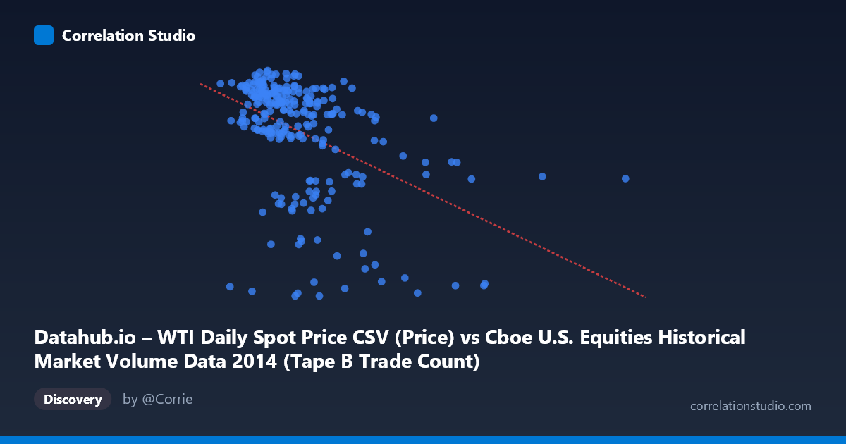
Relationship Overview The scatterplot reveals a moderate negative relationship between WTI daily spot prices (X-axis) and Cboe U.S. Equities Tape B trade counts (Y-axis) across 2014. The linear regression equation (y = -8.29×10⁻⁵x + 111.54) confirms that as oil prices increase, Tape B trade counts tend to decline. Visually, the data forms a somewhat diffuse cloud with a discernible downward slope, though considerable scatter is evident throughout. Notably, the distribution appears to concentrate in two rough zones: a dense cluster of higher trade counts (roughly 90–108) at lower-to-mid oil price ranges, and a sparser band of lower trade counts (roughly 54–65) spread more broadly across the price spectrum.
Correlation Strength and Statistical Significance The correlation coefficient of r = -0.4546 indicates a moderate negative association, but the explanatory power is limited: r² = 0.2067 means only ~20.7% of the variance in Tape B trade counts is explained by WTI prices, leaving nearly 80% attributable to other factors. The 95% confidence interval of [-0.5474, -0.3507] is entirely negative and does not cross zero, suggesting directional reliability, and the p-value of 2.953×10⁻¹⁴ confirms this correlation is highly statistically significant given the sample of 252 paired observations drawn from a population of 3,686. However, statistical significance here is partly a function of sample size and should not be conflated with practical or economic significance. Critically, Granger causality tests in both directions fail to reach significance (X→Y: F=1.17, p=0.312; Y→X: F=0.51, p=0.602), meaning neither variable demonstrably predicts the other temporally at a 2-period lag — the correlation may be coincidental or driven by shared underlying dynamics rather than any directional causal mechanism.
Notable Patterns, Clusters, and Outliers The scatterplot exhibits a striking bimodal or stratified structure in the Y-axis. Trade counts cluster heavily in the 95–108 range and again in the 54–66 range, with relatively few observations in between. This gap suggests the relationship may not be purely continuous or linear — there may be discrete market regimes or structural breaks at play. Several outliers are apparent: points like (478,251; 55.97) and (559,868; 82.33) represent unusually high oil prices paired with low trade counts, pulling the regression line noticeably. The point (176,548; 107.95) stands out as a maximum Tape B trade count at a relatively low oil price. The lower-trade-count cluster appears to span a wide range of oil prices, weakening the linear model's descriptive adequacy.
Confounding Factors and Caveats Several important caveats apply. 2014 was a structurally unusual year for oil markets — WTI prices began around $95/barrel and collapsed sharply to ~$55 by year-end, driven by OPEC supply decisions and surging U.S. shale production. This temporal drift means the X-variable is not randomly distributed but follows a strong downward trend, which could create spurious correlation with any market variable that changed concurrently. Tape B trade counts reflect equity trading in NYSE-listed securities on non-primary exchanges — their behavior is influenced by algorithmic trading patterns, volatility regimes, regulatory changes (e.g., Reg NMS dynamics), and overall market sentiment, none of which are captured here. The apparent bimodal distribution in trade counts may reflect seasonal effects, specific market events, or exchange-level structural changes unrelated to oil pricing. Additionally, the axes appear to be mislabeled in the source metadata (dataset names are swapped between X and Y descriptions), warranting careful verification before drawing domain-specific conclusions.
Actionable Insights and Further Investigation Given the moderate correlation but absent Granger causality, this relationship warrants skepticism about direct mechanistic linkage. Analysts should consider: (1) controlling for time as a covariate to determine whether the correlation persists after accounting for the shared 2014 downward trend in oil prices; (2) testing for structural breaks in the Tape B trade count series around key oil market events (e.g., OPEC's November 2014 decision); (3) expanding the lag window in Granger tests beyond 2 periods, as energy-equity market interactions may operate on longer horizons; (4) exploring whether the bimodal Y-distribution corresponds to identifiable calendar periods or volatility regimes using a time-series overlay; and (5) examining other equity market indicators (VIX, overall volume, sector-specific flows) alongside oil prices to build a more complete multivariate model that could meaningfully explain the remaining ~79% of variance in Tape B trade activity.
X dataset: Cboe U.S. Equities Historical Market Volume Data 2014
Y dataset: Datahub.io – WTI Daily Spot Price CSV
Part of experiment: Daily - Cboe U.S. Equities Historical Market Volume Data 2014 vs Datahub.io – WTI Daily Spot Price CSV