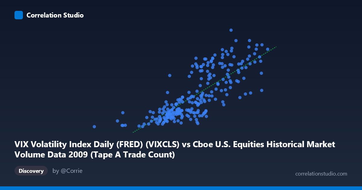
VIX Volatility Index Daily (FRED) (VIXCLS) vs Cboe U.S. Equities Historical Market Volume Data 2009 (Tape A Trade Count)
- Pearson correlation (r)
- 0.7838
- Spearman correlation
- 0.8148
- p-value
- 0
- Sample size (n)
- 252
- 95% confidence interval
- 0.731 to 0.8272
- Granger causality
- None
- Granger optimal lag
- 1
AI analysis
Analysis: VIX Volatility Index vs. Cboe Tape A Trade Count (2009)
Relationship Overview
The scatterplot reveals a moderately strong positive relationship between the VIX Volatility Index and Tape A Trade Count across 252 trading days in 2009. As VIX values rise — indicating greater market fear and implied volatility — the number of Tape A trades tends to increase substantially. This is intuitively consistent with market microstructure theory: elevated volatility drives heightened trading activity as investors rebalance, hedge, and react to rapidly shifting price signals. The linear regression equation (y = 1.83×10⁻⁵x + 1.693) suggests that for each unit increase in trade count, VIX rises by a small but meaningful increment, though the axis orientation means interpretation runs from trade volume predicting VIX levels.
Correlation Strength and Statistical Significance
The correlation of r = 0.784 is robust and statistically significant (p ≈ 0), with a tight 95% confidence interval of [0.731, 0.827], indicating high precision in the estimate given the large population of N = 3,232. The r² = 0.614 tells the more sobering story: roughly 61.4% of variance in VIX is explained by Tape A trade count, leaving nearly 39% attributable to other factors. This is a meaningful but incomplete explanatory relationship. Critically, Granger causality tests reveal no significant predictive directionality in either direction — neither X→Y (F = 0.352, p = 0.554) nor Y→X (F = 0.186, p = 0.667) — meaning that past values of one variable do not reliably help forecast the other at a one-period lag. The correlation is therefore contemporaneous rather than predictive, a crucial distinction for any trading or risk management application.
Patterns, Clusters, and Outliers
The scatterplot shows a visible bimodal clustering structure. A dense cluster sits in the lower-left region (trade counts roughly 19–27, VIX approximately 1.0M–1.8M), likely corresponding to calmer mid-to-late 2009 market conditions as volatility normalized following the 2008 financial crisis. A second, more dispersed cluster occupies the upper-right (VIX 30–55+, higher trade counts), reflecting the elevated volatility environment of early 2009. Several notable outliers appear at extreme VIX values (above 45–56), including points near (2,149,162, 52.62) and (2,320,189, 52.65), which sit at the upper boundary and may represent specific crisis-driven trading days. The point at (362,081, 19.47) is a conspicuous low-volume, low-VIX outlier well separated from the main cloud, potentially reflecting a holiday-shortened or anomalous trading session.
Confounding Factors and Caveats
Several important caveats temper interpretation. 2009 is a structurally unusual year — it spans the tail of the Global Financial Crisis and a historic market recovery, meaning the elevated volatility-volume co-movement may reflect a specific crisis regime rather than a generalizable relationship. Secular trends (both VIX and volume trended downward through 2009) could artificially inflate the correlation through shared time-series drift, a classic spurious correlation risk. The Granger non-causality finding reinforces that this may be a common-factor relationship — both variables responding simultaneously to macro news shocks — rather than one driving the other. Additionally, Tape A specifically covers NYSE-listed securities, so the relationship may not generalize to Tape B or C venues, and algorithmic trading patterns in 2009 differ substantially from contemporary markets.
Actionable Insights and Further Investigation
Despite the Granger non-causality finding, the strong contemporaneous correlation (r = 0.784) suggests VIX and Tape A volume serve as coincident indicators of market stress, useful for real-time risk dashboards rather than predictive models. Practitioners should investigate whether longer lag structures (beyond the single period tested) reveal delayed Granger causality, and whether regime-switching models better capture the two apparent clusters than a single linear fit. Extending the analysis across multiple years would test whether this relationship is stable or crisis-specific. Finally, decomposing trade count by participant type (market makers vs. institutional vs. retail) could isolate which trading behavior most tightly couples with VIX, offering more precise insights into volatility-driven market dynamics.
X dataset: Cboe U.S. Equities Historical Market Volume Data 2009
Y dataset: VIX Volatility Index Daily (FRED)
Part of experiment: Daily - Cboe U.S. Equities Historical Market Volume Data 2009 vs VIX Volatility Index Daily (FRED)