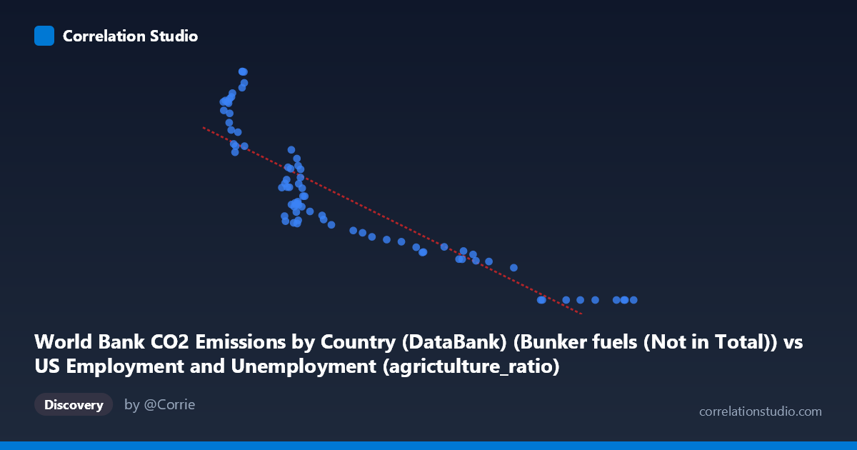
World Bank CO2 Emissions by Country (DataBank) (Bunker fuels (Not in Total)) vs US Employment and Unemployment (agrictulture_ratio)
- Pearson correlation (r)
- -0.8766
- Spearman correlation
- -0.9207
- p-value
- 0
- Sample size (n)
- 80
- 95% confidence interval
- -0.9193 to -0.8136
- Granger causality
- None
- Granger optimal lag
- 10
AI analysis
Analysis of CO2 Bunker Fuel Emissions vs. US Agricultural Employment Ratio
Relationship Overview
The scatterplot reveals a strong negative relationship between World Bank CO2 emissions from bunker fuels and the US agricultural employment ratio, spanning annual observations from 1941 to 2020. As bunker fuel CO2 emissions increase (X-axis, ranging from roughly 2,095 to 9,250 units), the agricultural employment ratio (Y-axis, 0 to ~1,592) declines substantially. The linear regression equation y = -0.197x + 1,543.56 captures this downward trajectory, and visually the data follow a coherent arc from the upper-left (low emissions, high agricultural ratio) to the lower-right (high emissions, near-zero agricultural ratio). Both variables are almost certainly driven by the same underlying historical force — the long-run economic modernization of the post-WWII era — making this a textbook case of a shared temporal trend rather than a direct causal mechanism.
Correlation Strength and Statistical Framing
The Pearson correlation of r = -0.877 is statistically strong and negative, with R² = 0.769, meaning approximately 76.8% of the variance in the agricultural employment ratio is statistically accounted for by variation in bunker fuel emissions within this sample. The 95% confidence interval of [-0.919, -0.814] is narrow and entirely negative, confirming robust certainty about the direction and magnitude of the association. The p-value of effectively 0 (given n = 80) rules out chance as an explanation for this pattern. However, the Granger causality results tell a critically different story: neither X→Y (F = 0.93, p = 0.51) nor Y→X (F = 1.22, p = 0.30) reaches significance at any conventional threshold, even at an optimal lag of 10 periods. This means that neither variable temporally predicts the other beyond what a simple time trend would explain — the correlation reflects co-movement through time, not predictive or mechanistic linkage.
Notable Patterns, Clusters, and Outliers
Several distinct clusters are visible. A dense concentration of points appears in the X range of ~2,100–3,900 paired with Y values of ~500–1,600, corresponding to earlier decades (1940s–1970s) when agricultural employment was still meaningful and bunker emissions were lower. A sparser cluster at X 6,000 shows Y values collapsing toward zero, reflecting the modern era. Notably, multiple data points have Y = 0 (e.g., at X values of 7,658; 8,073; 8,320; 8,580; 8,950; 9,080; 9,100; 9,250), suggesting the agricultural ratio effectively reached a floor — this compression at zero introduces a ceiling/floor effect that may slightly inflate the linear R². The relationship also appears to flatten nonlinearly at high X values, hinting that a logarithmic or segmented regression might better characterize the full trajectory than a strictly linear model.
Confounding Factors and Caveats
The most significant caveat is shared temporal trend confounding: both variables are annual time-series tracking secular post-war trends. Bunker fuel emissions rose steadily with global trade expansion, while US agricultural employment declined as mechanization and economic diversification advanced — two entirely independent processes that happen to move in opposite directions over the same 80-year window. This is a near-perfect example of a spurious correlation driven by time. Additionally, the dataset labels contain a potential metadata mismatch — "Bunker fuels (Not in Total)" are international shipping/aviation fuels, which have no plausible direct mechanism affecting US domestic farm employment. The column sourcing also appears cross-joined between two different datasets (US Employment and World Bank CO2), warranting verification that the join keys (likely by year) are correctly aligned.
Actionable Insights and Further Investigation
Given the absence of Granger causality, analysts should detrend both series (e.g., via first-differencing or HP filtering) before drawing any inferential conclusions — the raw correlation is almost entirely an artifact of shared time trends. Future investigation should test whether the correlation survives detrending, and whether other confounders (GDP growth, urbanization rate, global trade volume) absorb the residual association. A structural break analysis around major events (1970s oil shocks, 1990s globalization acceleration) could reveal whether the relationship changed character across sub-periods. Finally, if the research goal is understanding agricultural employment decline, variables with established mechanistic links — farm mechanization rates, rural-urban migration, agricultural productivity indices — would yield far more explanatory and actionable models than bunker fuel emissions.
X dataset: US Employment and Unemployment
Y dataset: World Bank CO2 Emissions by Country (DataBank)
Part of experiment: Yearly - US Employment and Unemployment vs World Bank CO2 Emissions by Country (DataBank)