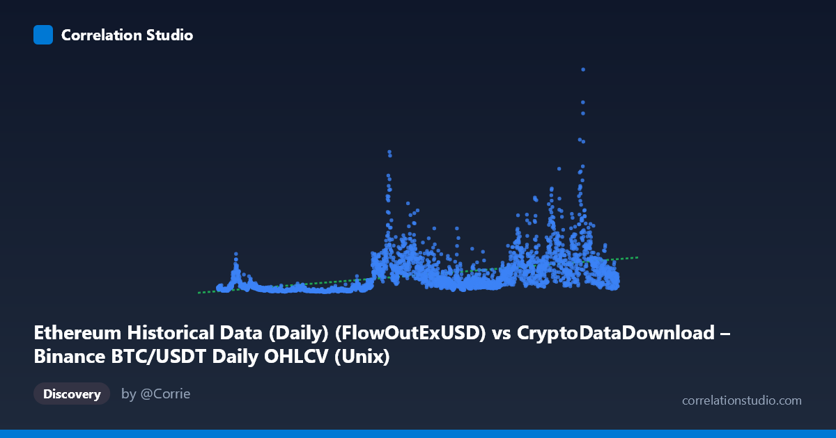
Ethereum Historical Data (Daily) (FlowOutExUSD) vs CryptoDataDownload – Binance BTC/USDT Daily OHLCV (Unix)
- Pearson correlation (r)
- 0.4792
- Spearman correlation
- 0.6385
- p-value
- 0
- Sample size (n)
- 3191
- 95% confidence interval
- 0.452 to 0.5055
- Granger causality
- None
- Granger optimal lag
- 10
- Time coverage
- 2017-08-17 to 2026-05-20
AI analysis
Analysis: Time (X) vs. Metric Value (Y)
1. Overview of the Relationship
The scatterplot plots a timestamp variable (labeled as Ethereum FlowOutExUSD, though the values are clearly Unix timestamps spanning 2017–2026) against a second variable (labeled as a Unix timestamp column, but with values ranging into the billions — inconsistent with raw timestamps, suggesting a mislabeled metric such as transaction volume, gas fees, or dollar-denominated flow). Treating X as time and Y as some market/network magnitude metric, the chart shows a positive but noisy upward drift: values tend to be low in the 2017–2020 period and generally larger (with high volatility) from 2021 onward, consistent with the historical growth trajectory of crypto markets.
2. Strength, Direction, and Statistical Confidence
The Pearson correlation of r = 0.479 indicates a moderate positive linear relationship. However, r² = 0.230 means only about 23% of the variance in Y is explained by X (time) — the remaining ~77% is driven by other factors, cyclical behavior, or noise. The 95% CI [0.452, 0.506] is tight and does not cross zero, and the p-value is effectively 0, so we can be confident the positive association is real and not due to sampling noise — but statistical significance here reflects the large sample size (n=3,191) more than practical predictive strength. Critically, the Granger causality tests show no significant predictive direction in either direction (X→Y: p=0.22; Y→X: p=0.23). This means that despite the contemporaneous correlation, past values of one series do not help forecast future values of the other beyond what each series' own history provides — the relationship is likely driven by a shared underlying trend (e.g., overall crypto market growth) rather than a causal lead-lag dynamic.
3. Patterns, Clusters, and Non-linearity
The data shows clear temporal clustering: a dense low-value cluster in 2017–2020 (Y mostly under 200M) and a more dispersed, higher-variance cluster from 2021 onward, with values spiking above 1B–7B during what appear to be bull-market peaks (e.g., early-to-mid 2021, 2024–2025). This produces a fan-shaped/heteroskedastic pattern — variance in Y increases substantially with X — which violates linear regression assumptions and explains why Spearman's rank correlation exceeds Pearson's r. This strongly suggests a non-linear or multiplicative relationship (e.g., exponential growth, log-normal distribution of Y) rather than a simple linear trend. Several extreme outliers (Y 3–7B) sit far above the regression line and likely correspond to specific market events (halving cycles, ETF approvals, or major volatility episodes) rather than steady-state behavior.
4. Confounding Factors and Caveats
Several caveats limit interpretation: (1) Metadata inconsistency — X is described as an Ethereum flow metric but contains timestamp values, while Y is labeled as a Unix timestamp column but contains large monetary-scale values; the axis labels appear swapped or mismatched with the underlying dataset descriptions, so conclusions about "which variable" is driving the relationship should be treated cautiously. (2) Because X is essentially a time index, any correlation with Y mostly reflects a shared secular trend (overall crypto market growth) rather than a meaningful bivariate relationship between two independent phenomena. (3) The extreme right-skew in Y (mean $569M vs. stdev $637M) suggests the data are far from normally distributed, further undermining the appropriateness of Pearson's r and linear regression. (4) Known confounds in crypto markets — halving cycles, regulatory announcements, macro liquidity conditions — could simultaneously drive both variables without any direct link between them.
5. Recommendations for Further Investigation
- Clarify variable definitions: verify axis/column mappings before drawing substantive conclusions, since the current labels are internally inconsistent. - Log-transform Y (and possibly detrend X) to stabilize variance and re-run correlation/regression — given the log-normal-looking distribution, a log-linear or polynomial model will likely fit much better than the current linear model. - Segment by market regime (bull/bear cycles, halving periods) rather than treating the full 2017–2026 span as homogeneous, since pooling regimes with very different volatility levels inflates apparent correlation while obscuring regime-specific dynamics. - Given the null Granger causality result, avoid using one series to forecast the other in a lead-lag trading or modeling strategy; instead, treat both as driven by common external factors (e.g., BTC price cycles, macro liquidity) and consider a multivariate model that explicitly includes those drivers. - Consider rolling-window correlation analysis to check whether the relationship strengthens/weakens across specific sub-periods (e.g., 2021 bull run vs. 2022 bear market), which would clarify whether the moderate aggregate r is masking stronger regime-specific relationships.
X dataset: CryptoDataDownload – Binance BTC/USDT Daily OHLCV
Y dataset: Ethereum Historical Data (Daily)
Part of experiment: Bitcoin - CryptoDataDownload – Binance BTC/USDT Daily OHLCV vs Ethereum Historical Data (Daily)