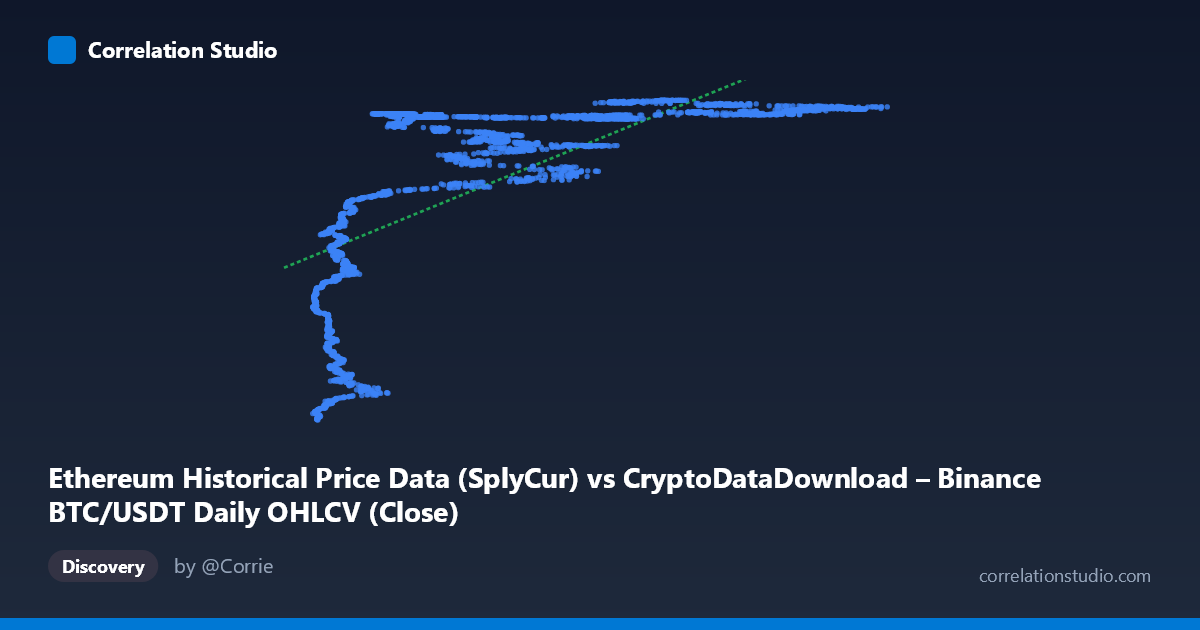
Ethereum Historical Price Data (SplyCur) vs CryptoDataDownload – Binance BTC/USDT Daily OHLCV (Close)

Pearson correlation (r): 0.6738
Spearman correlation: 0.8228
p-value: 0
Sample size (n): 3191
95% confidence interval: 0.6544 to 0.6924
Granger causality: None
Granger optimal lag: 10
Time coverage: 2017-08-17 to 2026-05-20

AI analysis

Analysis of the Relationship Between X and Y Variables

1. Overview of the Visualization

The scatterplot depicts a positive but clearly non-linear relationship between the X variable (labeled as "SplyCur," ranging from ~3,189 to ~124,659) and the Y variable (price-like values ranging from ~94M to ~122M). The data shows a distinctive pattern: at low X values (roughly 3,000–15,000), Y values are compressed into a lower band (~94M–113M), but Y rises very steeply and then plateaus into a tight, saturated band above ~120M once X exceeds approximately 20,000–25,000. This produces a shape resembling a logarithmic or saturating curve rather than a straight line — a classic "rapid rise then ceiling" pattern.

2. Strength, Direction, and Statistical Confidence

The Pearson correlation (r = 0.674) indicates a moderately strong positive linear relationship, with r² = 0.454 meaning the linear model explains only about 45% of the variance in Y — leaving more than half unexplained by a straight-line fit. The 95% CI [0.654, 0.692] is narrow, and p ≈ 0 confirms the correlation is highly statistically significant and not due to chance, aided by the large sample size (n = 3,191). However, statistical significance here reflects precision, not necessarily linear adequacy — the note that Spearman ρ exceeds Pearson r is a strong signal that a monotonic non-linear model (log or polynomial) would fit the data better than the linear one, consistent with the visual "elbow" pattern in the plot.

Critically, the Granger causality tests show no significant predictive direction in either direction (X→Y: p = 0.916; Y→X: p = 0.383). This means that despite the strong contemporaneous correlation, neither variable's past values help forecast the other's future values in a time-series sense. This is an important caveat: the relationship, while strong, does not indicate that movements in X cause or precede movements in Y (or vice versa) — they may instead be jointly driven by a shared underlying trend (e.g., overall market growth/time).

3. Notable Patterns and Features

The scatterplot shows several distinguishing features: - Compressed low-X cluster: A tight cluster of points with X < 15,000 and Y values spanning 94M–113M, representing steep sensitivity — small changes in X correspond to large swings in Y in this region. - Saturation/ceiling effect: For X 25,000, Y values cluster tightly near the top of the range (118M–122M), with diminishing sensitivity — increases in X produce little further change in Y. - A steep transition zone around X = 15,000–25,000, where Y climbs rapidly, forming the "elbow" of a logarithmic curve. - No obvious outliers stand out as violating the overall pattern; scatter is heavier (more vertical spread) at low X and compresses at high X, suggesting heteroscedasticity — variance in Y is not constant across the range of X.

4. Confounding Factors and Caveats

Both variables are derived from cryptocurrency price/supply metrics (BTC/USDT close price for Y; an Ethereum-labeled "SplyCur" column, though metadata inconsistently references BTC data as well — suggesting possible mislabeling or data-merging issues that should be verified). Because both series are time-indexed financial data over a multi-year period (2017–2026) with well-documented long-term uptrends, the correlation is very likely driven by a shared temporal trend (both assets have appreciated over time) rather than a direct causal or structural relationship. This is a common pitfall in time-series correlation analysis — "spurious regression" from co-integrated or trending series. The lack of Granger causality reinforces that these are likely two variables riding a common macro trend (bull markets, overall crypto sentiment, liquidity cycles) rather than one driving the other.

5. Suggestions for Further Investigation

1. Verify data integrity/labeling — the axis metadata mixes references to both BTC and ETH data; confirm which asset each column truly represents before drawing asset-specific conclusions. 2. Fit non-linear models (logarithmic, power, or piecewise/segmented regression) given the clear elbow shape and the Spearman-vs-Pearson discrepancy — this should substantially improve explained variance. 3. De-trend or difference the series (e.g., use returns/log-returns instead of levels) before testing correlation or Granger causality, since raw price levels in trending markets often produce misleading correlation strength. 4. Test for cointegration (e.g., Engle-Granger or Johansen test) given both are non-stationary financial time series — this would be more appropriate than raw correlation/Granger-on-levels. 5. Segment analysis by time period (e.g., by year or market regime) to check whether the strength/shape of the relationship is stable or driven by specific bull/bear cycles.

X dataset: CryptoDataDownload – Binance BTC/USDT Daily OHLCV

Y dataset: Ethereum Historical Price Data

Part of experiment: Bitcoin - CryptoDataDownload – Binance BTC/USDT Daily OHLCV vs Ethereum Historical Price Data