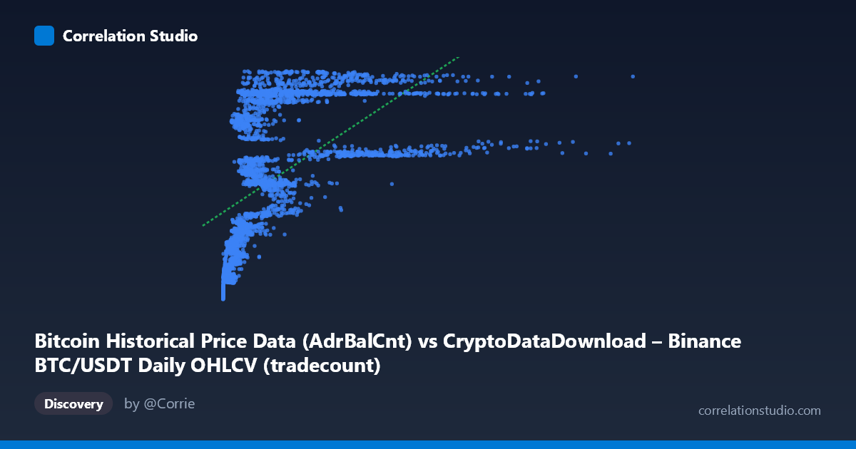
Bitcoin Historical Price Data (AdrBalCnt) vs CryptoDataDownload – Binance BTC/USDT Daily OHLCV (tradecount)
- Pearson correlation (r)
- 0.5532
- Spearman correlation
- 0.7826
- p-value
- 0
- Sample size (n)
- 3191
- 95% confidence interval
- 0.5287 to 0.5769
- Granger causality
- None
- Granger optimal lag
- 10
AI analysis
Analysis: Bitcoin AdrBalCnt vs. Tradecount Relationship
1. What the Visualization Reveals
The scatterplot shows a moderate positive relationship between the X variable (labeled "AdrBalCnt" but actually appears to be a price/value metric given its scale) and Y (tradecount). The data shows a clear pattern where low-X observations cluster tightly around Y values of 19-30 million, while higher-X values correspond to a wider spread of Y values reaching up to ~57 million. This fan-shaped or curved pattern—rather than a uniform linear scatter—suggests the relationship strengthens and changes character as X increases, consistent with the note that Spearman's rank correlation exceeds Pearson's r.
2. Strength, Direction, and Statistical Confidence
The correlation coefficient (r = 0.553) indicates a moderate positive relationship, but r² = 0.306 reveals that only ~31% of the variance in tradecount is explained by X, leaving roughly 69% attributable to other factors, noise, or non-linear dynamics not captured by this simple linear fit. The tight 95% confidence interval [0.529, 0.577] combined with p ≈ 0 confirms this correlation is highly statistically reliable and not a product of chance—but statistical significance here reflects the large sample size (n=3,191) more than practical predictive strength. Critically, the Granger causality tests show no significant predictive direction in either direction (X→Y: p=0.078; Y→X: p=0.474) at the optimal 10-period lag. This means neither variable meaningfully "leads" the other in time—the correlation is likely contemporaneous/structural (both driven by overall market growth) rather than one causing or forecasting the other.
3. Notable Patterns and Non-linearity
Several features stand out: - Compressed low-end cluster: Numerous points with X < 500,000 show Y values tightly bounded between ~19M-33M, suggesting a floor effect or early-period data density. - Fan/heteroscedastic spread: As X increases beyond ~1M, the Y-range widens dramatically (from ~36M to ~57M), indicating variance is not constant across X — a violation of standard linear regression assumptions. - Possible saturation/ceiling: Y values seem to plateau near 55-57M even as X grows into the millions, hinting at a logarithmic or asymptotic relationship rather than linear. - Extreme X outlier: The max X value (15,364,010) is far beyond the mean+stdev range of most points, and may be exerting outsized leverage on the linear fit.
The suggestion that a logarithmic or polynomial transformation of X would fit better is well-supported visually—this pattern (rapid Y growth at low X, then flattening) is classic log-shaped behavior.
4. Confounding Factors and Caveats
- Time-trend confounding: Both variables likely trend upward over the 2017-2026 period as Bitcoin/Binance matured, inflating correlation without direct causal linkage (spurious correlation via a shared time trend). - Metric mismatch: The labeling is inconsistent (X axis described as both "AdrBalCnt" and price OHLCV data)—this ambiguity should be resolved before drawing domain conclusions. - Non-stationarity: Financial/network time series are typically non-stationary; Granger causality and Pearson correlation both assume properties (stationarity, linearity) that may be violated here, potentially explaining the weak/insignificant Granger results despite decent contemporaneous correlation. - Autocorrelation: Daily crypto data is highly autocorrelated, which can artificially inflate significance (low p-values) even for a modest r².
5. Actionable Recommendations
1. Re-fit with log(X) or polynomial terms — given the fan pattern and Spearman Pearson signal, a log-linear model will likely substantially improve R². 2. Test for stationarity (ADF/KPSS tests) and consider differencing or detrending both series before re-running correlation and Granger tests, to rule out spurious trend-driven correlation. 3. Segment the analysis by time period (e.g., pre/post major Bitcoin bull runs) to check if the relationship is stable or regime-dependent. 4. Clarify variable definitions — confirm what X actually represents (price vs. address balance count) since this fundamentally changes interpretation. 5. Investigate the extreme X outlier for data integrity issues, and consider robust regression (e.g., Theil-Sen) to reduce leverage effects.
X dataset: CryptoDataDownload – Binance BTC/USDT Daily OHLCV
Y dataset: Bitcoin Historical Price Data
Part of experiment: Bitcoin - CryptoDataDownload – Binance BTC/USDT Daily OHLCV vs Bitcoin Historical Price Data