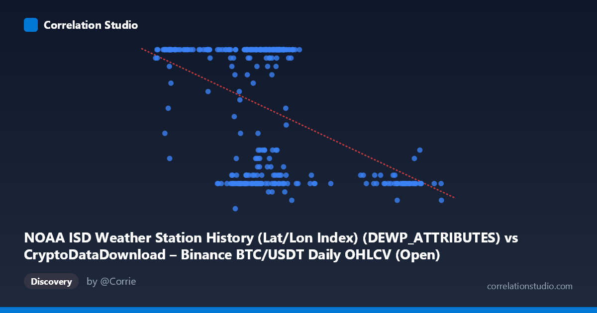
NOAA ISD Weather Station History (Lat/Lon Index) (DEWP_ATTRIBUTES) vs CryptoDataDownload – Binance BTC/USDT Daily OHLCV (Open)
- Pearson correlation (r)
- -0.4705
- Spearman correlation
- -0.3122
- p-value
- 0
- Sample size (n)
- 355
- 95% confidence interval
- -0.5478 to -0.3853
- Granger causality
- None
- Granger optimal lag
- 1
AI analysis
Analysis: NOAA Weather Station Index vs. Binance BTC/USDT Open Price
Important preliminary note: The column labeling here appears mismatched or mislabeled — the "X-axis" is described as a weather station attribute field but its values (39,568 to 106,133) resemble price data, while "Y" (5-24 range) looks like a bounded categorical or index-like variable, not an "Open" price for BTC/USDT (which would range in the thousands to tens of thousands of dollars). This suggests the axis labels/dataset descriptions may have been swapped or corrupted during data pairing. Any interpretation should be treated cautiously, and the following analysis addresses the statistical relationship as given, independent of the questionable semantic labels.
1. What the Visualization Reveals The scatterplot shows a negative, moderate-strength linear relationship between X and Y. As X increases, Y tends to decrease, though the relationship is noisy rather than a clean trend. The Y variable appears to cluster heavily at two levels — a dense band near Y=24 (the apparent ceiling) and a secondary cluster around Y=8-12 — suggesting Y may behave as a semi-discrete or capped variable rather than a continuous one. X values below ~70,000 disproportionately populate the Y=24 cluster, while X values above ~90,000 consistently fall in the low Y band (8-11).
2. Strength, Direction, and Statistical Confidence The correlation coefficient (r = -0.47) indicates a moderate negative relationship. The r² of 0.221 means only about 22% of the variance in Y is explained by X — the majority (78%) is driven by other factors or noise. The 95% CI [-0.548, -0.385] is reasonably tight and entirely negative, and the p-value of ~0 confirms this correlation is statistically significant and not due to chance, given the large sample (n=355). However, statistical significance here reflects sample size more than practical strength — with r² this low, X is a weak-to-moderate predictor of Y at best, not a reliable one-to-one driver. Critically, Granger causality tests show no significant predictive direction in either direction (X→Y: p=0.708; Y→X: p=0.259). This means despite the contemporaneous correlation, neither variable helps forecast future values of the other — the relationship, if genuine, is not temporally causal in this lagged sense; it may be simultaneous, coincidental, or driven by a shared external factor.
3. Notable Patterns and Outliers The data shows a distinctly bimodal/clustered structure rather than a smooth continuous scatter: - A dominant cluster at Y=24 spanning X≈41,000–73,000 - A lower cluster at Y=7-12 that appears at both low X (~42,000-43,000, e.g., the point (42847.99, 11.00)) and high X (~90,000-100,000) - Sparse mid-range Y values (17, 19, 21-23) act as transitional points
This clustering pattern — rather than a diffuse cloud — suggests the relationship may be driven by a threshold effect or regime-switching behavior (e.g., Y=24 as a ceiling/cap value) rather than a true linear mechanism. The presence of low-Y points at both low and high X extremes weakens the linear model's fit and explains the modest r².
4. Confounding Factors and Caveats Given the likely mislabeled/mismatched dataset pairing (weather station attributes paired with cryptocurrency price fields), any "relationship" may be a spurious correlation arising from incidental alignment of unrelated time series (a common risk when merging datasets by date/index without validating semantic meaning). Even taking the data at face value, unmeasured confounders (time-of-year effects, data preprocessing/binning that created the Y ceiling at 24, or shared temporal trends) could produce this pattern without genuine causal linkage. The linear regression (R²=0.221) is a poor fit given the visible clustering — a linear model likely misrepresents the true (possibly categorical or threshold-based) structure.
5. Recommendations 1. Verify data provenance and column mapping — confirm that X and Y are correctly sourced and that the "Open" price and "DEWPATTRIBUTES" labels are not swapped or corrupted, given the implausible value ranges. 2. Investigate the Y=24 ceiling — determine if this is a capped/clipped value (e.g., max index score) requiring censored regression or a different modeling approach. 3. Test non-linear/segmented models — given the clustering, consider a threshold, logistic, or piecewise regression rather than simple OLS. 4. Treat the correlation as non-causal — the Granger test results mean this relationship (if real) should not be used for forecasting one variable from the other. 5. Check for a lurking date-based confound — since both datasets are indexed to 2024 dates, examine whether both series independently trend with time (seasonality, price cycles) which could produce this correlation without direct interaction.
X dataset: CryptoDataDownload – Binance BTC/USDT Daily OHLCV
Y dataset: NOAA ISD Weather Station History (Lat/Lon Index)
Part of experiment: Bitcoin - CryptoDataDownload – Binance BTC/USDT Daily OHLCV vs NOAA ISD Weather Station History (Lat/Lon Index)