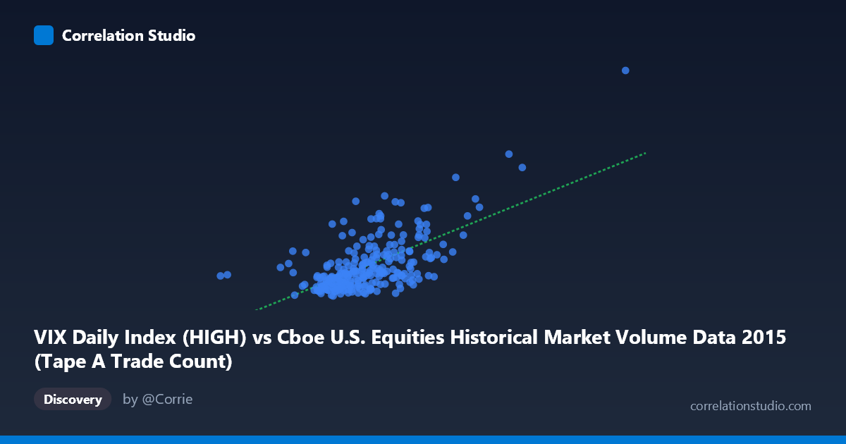
VIX Daily Index (HIGH) vs Cboe U.S. Equities Historical Market Volume Data 2015 (Tape A Trade Count)
- Pearson correlation (r)
- 0.6428
- Spearman correlation
- 0.5525
- p-value
- 0
- Sample size (n)
- 252
- 95% confidence interval
- 0.564 to 0.71
- Granger causality
- None
- Granger optimal lag
- 1
AI analysis
Scatterplot Analysis: VIX High vs. Tape A Trade Count (2015)
Relationship Overview The scatterplot reveals a moderate positive relationship between the VIX Daily Index High values and Cboe U.S. Equities Tape A Trade Count across 2015. As the VIX High increases — indicating greater expected market volatility — trade counts tend to rise correspondingly. This is intuitive: elevated volatility typically drives higher trading activity as market participants react to uncertainty, rebalance portfolios, or execute hedging strategies. The linear regression equation (y = 1.27035E-05x − 0.363214) confirms the positive slope, though the intercept's negative value suggests the relationship is only meaningful within the observed data range and should not be extrapolated far beyond it.
Correlation Strength and Statistical Significance With r = 0.6428, the correlation is moderate-to-strong and statistically significant (p ≈ 0, N = 3,302). The R² of 0.4132 means that approximately 41.3% of the variance in Tape A Trade Count is explained by VIX High values — a meaningful but incomplete explanation, with roughly 59% of variability attributable to other factors. The 95% confidence interval of [0.5640, 0.7100] is relatively tight, lending confidence that the true population correlation falls solidly in the moderate-to-strong range. However, the Granger causality results are notable: neither direction (X→Y: F = 0.0482, p = 0.826; Y→X: F = 0.0817, p = 0.775) shows significant temporal predictive power at a 1-period lag. This means that while the two variables are contemporaneously correlated, knowing yesterday's VIX High does not reliably predict today's trade count, and vice versa — suggesting the relationship is driven by shared simultaneous responses to market events rather than one variable leading the other.
Patterns, Clusters, and Outliers The data exhibits a fan-shaped or heteroscedastic dispersion — variance in trade counts appears to widen as VIX values increase, which is a common feature in volatility-driven financial data. At lower VIX High values (roughly 12–20), the trade counts are tightly clustered and relatively low, suggesting stable, low-volatility regimes produce predictable, subdued trading. A notable cluster of points exists in this lower-left region. At higher VIX values (25–53), the scatter broadens considerably, and several outliers are visible — particularly a point near VIX ~53 with a very high trade count, likely corresponding to the August 2015 market sell-off, a well-documented volatility spike. Points like (2247816.08, 38.06) and (2076907.15, 28.38) in the sample also suggest discrete high-activity events. The single extreme low-X outlier at (576208.00, 15.88) appears anomalous and may represent a data artifact or holiday-shortened session.
Confounding Factors and Caveats Several important caveats apply. First, 2015 was not a typical year — it included specific macro events (August China-driven selloff, Federal Reserve rate decisions) that simultaneously drove both volatility and volume, which could inflate the correlation artificially. Second, the axis labels appear swapped relative to their source datasets (VIX data described as the X-axis column but sourced from an equities volume dataset, and vice versa), which warrants careful verification of variable assignment before drawing causal conclusions. Third, trade count is an absolute measure not normalized for market size or time-of-day effects, which introduces noise. Finally, the heteroscedasticity observed suggests a linear model may not be the best fit — a log-linear or power-law transformation could yield a better-specified relationship and more stable residuals.
Actionable Insights and Further Investigation Practitioners should explore whether this correlation persists across multiple years to distinguish structural relationships from 2015-specific event effects. Given the Granger causality null results, intraday data (rather than daily lags) might reveal faster-acting predictive dynamics between volatility signals and trade execution. Decomposing Tape A Trade Count by trader type or trade size could clarify whether the correlation is driven by retail reactivity, algorithmic responses, or institutional hedging. Additionally, testing a log-transformed or piecewise regression model could better capture the apparent non-linearity at high VIX values. Finally, incorporating additional predictors (e.g., VIX term structure, S&P 500 returns, macroeconomic announcements) into a multivariate model would help account for the 58.7% of unexplained variance and provide a more robust forecasting framework.
X dataset: Cboe U.S. Equities Historical Market Volume Data 2015
Y dataset: VIX Daily Index
Part of experiment: Daily - Cboe U.S. Equities Historical Market Volume Data 2015 vs VIX Daily Index