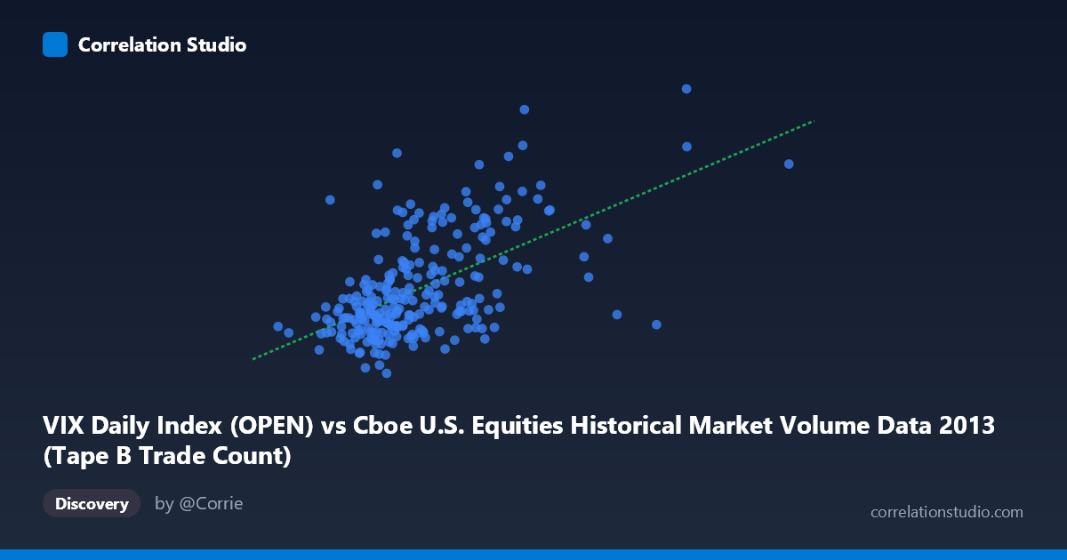
VIX Daily Index (OPEN) vs Cboe U.S. Equities Historical Market Volume Data 2013 (Tape B Trade Count)
- Pearson correlation (r)
- 0.5746
- Spearman correlation
- 0.5279
- p-value
- 0
- Sample size (n)
- 252
- 95% confidence interval
- 0.4855 to 0.6519
- Granger causality
- None
- Granger optimal lag
- 1
AI analysis
Analysis: VIX Daily Index (Open) vs. Tape B Trade Count (2013)
Relationship Overview The scatterplot reveals a moderate positive relationship between the VIX Daily Index open values and Tape B trade counts across U.S. equities exchanges in 2013. As VIX levels rise — indicating greater market uncertainty and implied volatility — Tape B trade counts tend to increase as well. This is broadly intuitive: elevated volatility environments typically drive higher trading activity as market participants react to uncertainty, reposition portfolios, or hedge exposures. The linear regression equation (y = 2.17347E-05x + 10.512) confirms the positive slope, though the modest coefficient suggests that VIX explains only a portion of trade count variation.
Correlation Strength and Statistical Framing The Pearson correlation of r = 0.5746 indicates a moderate positive association, but the more telling figure is r² = 0.3301, meaning VIX open levels explain only about 33% of the variance in Tape B trade counts. Roughly two-thirds of trade count variability stems from factors unrelated to VIX. The 95% confidence interval of [0.4855, 0.6519] is reasonably tight and does not cross zero, and the p-value of effectively 0 confirms the relationship is statistically significant across the sample of 252 daily paired observations drawn from a population of 3,780. However, statistical significance should not be conflated with practical predictive power — the relationship, while real, is far from deterministic. Critically, Granger causality analysis finds no significant predictive direction in either direction (X→Y: F = 0.6755, p = 0.412; Y→X: F = 0.1961, p = 0.658), meaning that past VIX values do not reliably predict future trade counts, and vice versa. This suggests the correlation reflects contemporaneous co-movement rather than a lead-lag causal mechanism.
Notable Patterns, Clusters, and Outliers The sample data reveals several interesting structural features. The bulk of observations cluster in a lower-left region with VIX values between roughly 130,000–200,000 and trade counts between 12–15, suggesting these represent "normal" 2013 market conditions with moderate volatility and routine trading volumes. A secondary cluster emerges at higher VIX values (210,000–250,000) with trade counts in the 15–17 range, consistent with periodic volatility spikes driving elevated activity. Several notable outliers are visible: the point near (241,064, 19.01) stands out with an unusually high trade count for its VIX level, as does the point near (327,004, 13.12), which shows a very high VIX open but a surprisingly low trade count — potentially representing a day when volatility was elevated but trading was muted, perhaps due to a holiday-adjacent session or a specific market structural event. These outliers could disproportionately influence the regression slope.
Confounding Factors and Caveats Several important caveats apply to this interpretation. First, dataset labeling warrants scrutiny: the X-axis is labeled as "VIX Daily Index (OPEN)" from the market volume dataset, while the Y-axis draws "Tape B Trade Count" from the VIX dataset — this cross-dataset sourcing could introduce alignment or definitional inconsistencies. Second, Tape B specifically covers NYSE American (formerly AMEX) and regional exchange securities, which may behave differently from broader market benchmarks, potentially weakening the VIX relationship compared to large-cap S&P 500-linked activity. Third, secular trends within 2013 — such as the May/June "taper tantrum" volatility episode — could be driving both variables simultaneously, creating a spurious or inflated correlation that is time-period specific. Finally, the absence of Granger causality at lag 1 does not rule out longer-lag relationships or non-linear dynamics that the linear model fails to capture.
Actionable Insights and Further Investigation Given the moderate but incomplete explanatory power and the absence of Granger causality, practitioners should avoid using VIX alone as a predictive trigger for Tape B trade volume. Instead, several follow-up analyses are warranted: (1) Extend the lag structure in Granger causality testing beyond lag 1 to check for delayed transmission effects; (2) Segment the data by volatility regime (e.g., VIX quartiles) to test whether the relationship strengthens nonlinearly during high-volatility episodes; (3) Include additional covariates such as overall market volume, S&P 500 returns, and day-of-week effects to build a more robust multivariate model; (4) Replicate across multiple years to determine whether the r = 0.57 relationship is stable or an artifact of 2013's specific volatility environment. The outlier near (327,004, 13.12) in particular deserves individual investigation to determine whether it represents a data anomaly or a genuinely informative extreme event.
X dataset: Cboe U.S. Equities Historical Market Volume Data 2013
Y dataset: VIX Daily Index
Part of experiment: Daily - Cboe U.S. Equities Historical Market Volume Data 2013 vs VIX Daily Index