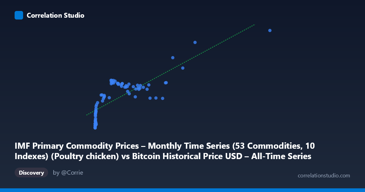
IMF Primary Commodity Prices – Monthly Time Series (53 Commodities, 10 Indexes) (Poultry chicken) vs Bitcoin Historical Price USD – All-Time Series (Habrador) (Price)
- Pearson correlation (r)
- 0.7958
- Spearman correlation
- 0.7949
- p-value
- 0
- Sample size (n)
- 83
- 95% confidence interval
- 0.7003 to 0.8633
- Granger causality
- None
- Granger optimal lag
- 1
AI analysis
Analysis: Bitcoin Price vs. Poultry (Chicken) Commodity Index
1. What the Visualization Reveals
The scatterplot shows a strongly non-linear, saturating relationship rather than a clean linear one. At low X values (roughly 0–100, representing the bulk of the 83 observations), Y climbs steeply from ~85 to ~106. Between X≈100–1000, Y rises more gradually and plateaus in the 104–116 range with a modest dip around X=770–950 (Y drops back to ~104). Only at very high X values (1000, a handful of points) does Y climb sharply again, up to the maximum of 148.38 at X=2452.18. The shape resembles a logarithmic or power curve, not a straight line, even though the reported regression is linear.
2. Strength, Direction, and Statistical Meaning
The linear correlation is strong and positive (r = 0.7958, r² = 0.6333), indicating that a simple linear model explains about 63% of the variance in Y — a substantial but incomplete fit, since 37% of variance is unexplained. The 95% CI [0.70, 0.86] is reasonably tight and excludes zero, and the p-value (~0) confirms this is not a chance finding. However, given the visibly curved pattern, a linear r may actually understate the true (monotonic/non-linear) association — a log-transform of X would likely yield a tighter fit and higher r².
Critically, the Granger causality tests show no significant predictive direction in either direction (X→Y: p=0.73; Y→X: p=0.55). This means that despite the strong contemporaneous correlation, neither series reliably helps forecast future values of the other using their own past lags. This is an important distinction: correlation ≠ prediction. The relationship may be driven by a shared underlying trend (e.g., both series drifting upward over the 2010–2017 period) rather than one causally leading the other.
3. Notable Patterns and Outliers
- Clustering: The vast majority of points sit at X<400 (early low-price Bitcoin era), producing a dense cluster where Y rises quickly with small X changes — this is the steepest part of the curve. - Plateau region: X=400–950 shows Y hovering in a narrow 104–116 band, suggesting diminishing sensitivity of Y to X in this range. - Dip anomaly: Around X=770–950, Y actually decreases slightly (to ~104), breaking the otherwise monotonic trend — this could reflect a genuine decoupling period or an artifact of sparse sampling. - High-leverage outliers: The three points above X=1000 (1089, 1230, 1402, 2452) with Y ranging 123–148 have outsized influence on the linear regression slope and r² — removing them could substantially change the fit.
4. Confounding Factors and Caveats
Both series span 2010–2017, a period when Bitcoin grew from near-zero to major bull-market territory, and global commodity indexes (including poultry) also experienced independent inflationary and supply-driven cycles. Any two time series with a general upward trend over time will show spurious positive correlation without any causal link — this is a classic time-series confounding issue. The lack of Granger causality supports the idea that shared time-trend (or a common macro driver like USD inflation, global liquidity, or simply calendar time) may be responsible for the correlation rather than a direct economic relationship between Bitcoin and chicken prices. Additionally, n=83 paired points is a small, likely monthly-aggregated sample relative to full Bitcoin's daily granularity, and the extreme skew in X (mean 321, stdev 405, max 2452) means the regression is heavily influenced by a few high-value points.
5. Suggestions for Further Investigation
- Detrend both series (e.g., differencing or removing linear time trends) before correlating, to test whether the relationship survives after removing common upward drift. - Log-transform X given the visibly saturating/logarithmic shape; refit regression and compare r². - Sensitivity/outlier analysis: Re-run correlation excluding the four X1000 points to check robustness. - Investigate the dip at X≈770–950 to determine if it's a real economic signal or noise. - Treat this pairing primarily as a statistical curiosity (likely spurious given no Granger causality) rather than an economically meaningful relationship — poultry commodity prices have no obvious mechanistic link to Bitcoin valuation.
X dataset: Bitcoin Historical Price USD – All-Time Series (Habrador)
Y dataset: IMF Primary Commodity Prices – Monthly Time Series (53 Commodities, 10 Indexes)
Part of experiment: Bitcoin - Bitcoin Historical Price USD – All-Time Series (Habrador) vs IMF Primary Commodity Prices – Monthly Time Series (53 Commodities, 10 Indexes)