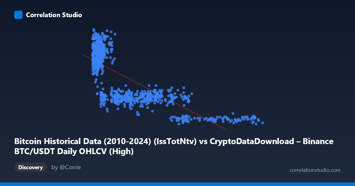
Bitcoin Historical Data (2010-2024) (IssTotNtv) vs CryptoDataDownload – Binance BTC/USDT Daily OHLCV (High)
- Pearson correlation (r)
- -0.7763
- Spearman correlation
- -0.7599
- p-value
- 0
- Sample size (n)
- 938
- 95% confidence interval
- -0.8005 to -0.7496
- Granger causality
- None
- Granger optimal lag
- 10
- Time coverage
- 2017-08-20 to 2026-05-20
AI analysis
Analysis: Bitcoin Issued Native Units vs. Daily High Price
1. What the Visualization Reveals
The scatterplot depicts a clear inverse, non-linear relationship between the X variable (issued native units, a proxy tied to Bitcoin's supply/network activity) and Y (daily high price). As X increases, Y decreases in a curved, decaying fashion rather than a straight line—prices drop steeply at low X values and then flatten out at high X values. This shape is more consistent with a power-law, logarithmic, or exponential decay relationship than a true linear one, even though a linear fit is reported.
2. Strength, Direction, and Statistical Confidence
The Pearson correlation of r = -0.7763 indicates a strong negative linear association, with r² = 0.6027 meaning the linear model explains about 60% of the variance in price—leaving a substantial 40% unexplained, likely due to the curvature evident in the data. The 95% confidence interval [-0.80, -0.75] is tight, and the p-value of ~0 confirms this relationship is highly statistically significant and not due to chance, given the large sample (n=938). However, the Granger causality results are critical: neither direction (X→Y or Y→X) shows significant predictive causality (p=0.33 and p=0.74 respectively). This means that despite the strong contemporaneous correlation, X does not temporally predict future Y, nor vice versa—the relationship is likely coincidental to a shared underlying driver (e.g., time/market cycle) rather than one variable causally driving the other in a forecastable way.
3. Notable Patterns and Outliers
The data clearly clusters into two regimes: a dense cluster at low X (roughly 3,000–15,000) where Y ranges widely from ~1,600 to 2,225 (high volatility in price at low issuance values), and a sparse tail at high X (60,000–125,000) where Y compresses tightly into a low range (425–950). This suggests heteroscedasticity—variance in Y is much higher at low X than at high X. The extreme values (X 100,000 paired with Y < 500) represent a handful of points that could disproportionately influence the linear r² and slope; these should be checked as potential leverage points. The curve's shape (steep drop then plateau) suggests a log or inverse transformation of X would likely produce a better linear fit.
4. Confounding Factors and Caveats
Both variables are derived from the same underlying asset (Bitcoin) and the same time series, so this is fundamentally an autocorrelated, non-independent relationship rather than two separate phenomena—"issued native units" likely tracks cumulative supply or block rewards, which mechanically increases over time as price has historically fluctuated across bull/bear cycles. This creates a spurious correlation risk: both variables trend with calendar time (2017–2026), so the negative correlation may simply reflect that supply grew steadily while price went through cycles, not a direct causal link. Time itself is a likely confounder, and the lack of Granger causality supports treating this as a co-trending artifact rather than a genuine predictive relationship.
5. Actionable Insights
For further investigation: (1) test non-linear fits (log-log, exponential) to better capture the curvature and likely improve on the 60% variance explained; (2) decompose both series by time period/halving cycle to check if the relationship holds within each cycle or is purely a between-cycle artifact; (3) given the null Granger causality, avoid using X to forecast Y (or vice versa) in any predictive model—instead, treat correlation as descriptive only; (4) investigate a third variable (e.g., calendar time, halving events, or macro market cycles) as the true common driver; and (5) examine the high-X outliers separately, as they may represent a distinct market regime (e.g., late-stage bear market) worth modeling independently.
X dataset: CryptoDataDownload – Binance BTC/USDT Daily OHLCV
Y dataset: Bitcoin Historical Data (2010-2024)
Part of experiment: Bitcoin - CryptoDataDownload – Binance BTC/USDT Daily OHLCV vs Bitcoin Historical Data (2010-2024)