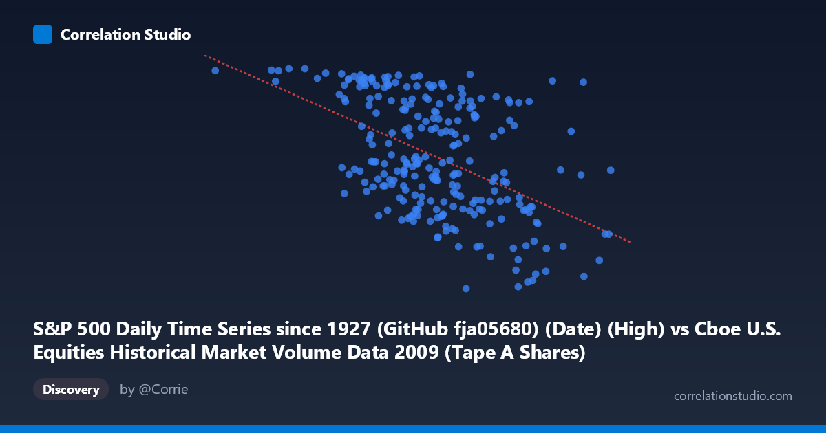
S&P 500 Daily Time Series since 1927 (GitHub fja05680) (Date) (High) vs Cboe U.S. Equities Historical Market Volume Data 2009 (Tape A Shares)
- Pearson correlation (r)
- -0.4969
- Spearman correlation
- -0.4915
- p-value
- 0
- Sample size (n)
- 252
- 95% confidence interval
- -0.5846 to -0.3978
- Granger causality
- X → Y
- Granger optimal lag
- 10
AI analysis
Analysis: S&P 500 Daily High vs. Cboe Tape A Share Volume (2009)
Relationship Overview
The scatterplot reveals a moderate negative relationship between the S&P 500 daily high price (X-axis) and Cboe Tape A share volume (Y-axis) across 2009. As the index traded at higher price levels, Tape A share volume tended to be lower, and conversely, during the market's distressed, lower-price periods early in 2009, trading volume was elevated. This pattern is broadly consistent with the market narrative of 2009: intense, high-volume panic selling near the March lows gave way to a grinding, lower-volume recovery rally through the second half of the year. The linear regression equation (y = −5.73×10⁻⁷x + 1208.09) captures this inverse slope, though the relationship is far from deterministic.
Correlation Strength, Direction, and Causality
The Pearson correlation of r = −0.497 indicates a moderate negative association. Critically, the R² of 0.247 means that only about 24.7% of the variance in Tape A share volume is explained by the S&P 500 daily high — leaving roughly three-quarters of volume variability unexplained by price level alone. The 95% confidence interval of [−0.585, −0.398] is meaningfully narrow and sits entirely in negative territory, and the p-value of effectively zero (against N = 3,232) confirms this is not a chance finding. The Granger causality result adds an important directional dimension: X (S&P 500 high) unidirectionally Granger-causes Y (Tape A volume) at an optimal lag of 10 trading periods (F = 1.96, p = 0.038), while the reverse direction fails to reach significance (p = 0.338). This suggests that price level changes tend to temporally precede volume shifts by approximately two calendar weeks, rather than volume leading price — a noteworthy asymmetry for market microstructure interpretation.
Notable Patterns, Clusters, and Outliers
The sample points reveal several structural features worth noting. There is a visible high-volume, low-price cluster (X roughly 105M–350M range on the date axis corresponding to early 2009, with Y values frequently above 1,050–1,130 shares), consistent with the bear-market bottom period. A contrasting low-volume, higher-price cluster emerges at higher X values (mid-to-late 2009 recovery), though with considerable scatter. Several notable outliers stand out: the point near (105,713,299, 1126.48) represents an extreme — the lowest price observation paired with very high volume — and points like (564,167,294, 699.09) and (606,087,715, 729.57) show anomalously low volume despite mid-range price levels, suggesting specific days with unusual activity suppression. The spread of Y values at any given X is wide, visually confirming the modest R².
Confounding Factors and Caveats
Several important caveats temper interpretation. Temporal autocorrelation is almost certainly present in both series — daily price and volume data are serially dependent, which can inflate apparent statistical significance even with a large N. The 2009 period is highly atypical, spanning a historic market bottom (March 9, 2009) and subsequent recovery, meaning the negative correlation may largely reflect this singular macro regime rather than a stable structural relationship. Cboe Tape A volume specifically captures NYSE-listed security trades, so this is not total market volume; compositional shifts in where trading occurred (fragmentation across venues was accelerating in 2009) could distort the signal. The Granger causality result, while statistically significant, has a relatively modest F-statistic (1.96) and should not be over-interpreted as strong economic causation — common drivers such as VIX (fear/volatility), institutional rebalancing cycles, and macro news flow likely confound both series simultaneously.
Actionable Insights and Further Investigation
Practitioners should investigate whether the relationship holds across different market regimes (bull vs. bear markets, pre/post-2008 crisis) to assess structural stability. Incorporating implied volatility (VIX) as a covariate in a multiple regression framework would likely absorb much of the currently unexplained 75.3% variance and clarify whether price level retains independent explanatory power for volume. The 10-period Granger lag warrants further examination — testing whether this lag corresponds to options expiration cycles or institutional reporting periods could yield actionable trading microstructure insights. Finally, expanding the analysis to all tape categories (B and C) and total consolidated volume would reveal whether the inverse price-volume dynamic is specific to large-cap NYSE-listed stocks or is a market-wide 2009 phenomenon.
X dataset: Cboe U.S. Equities Historical Market Volume Data 2009
Y dataset: S&P 500 Daily Time Series since 1927 (GitHub fja05680) (Date)
Part of experiment: Daily - Cboe U.S. Equities Historical Market Volume Data 2009 vs S&P 500 Daily Time Series since 1927 (GitHub fja05680) (Date)