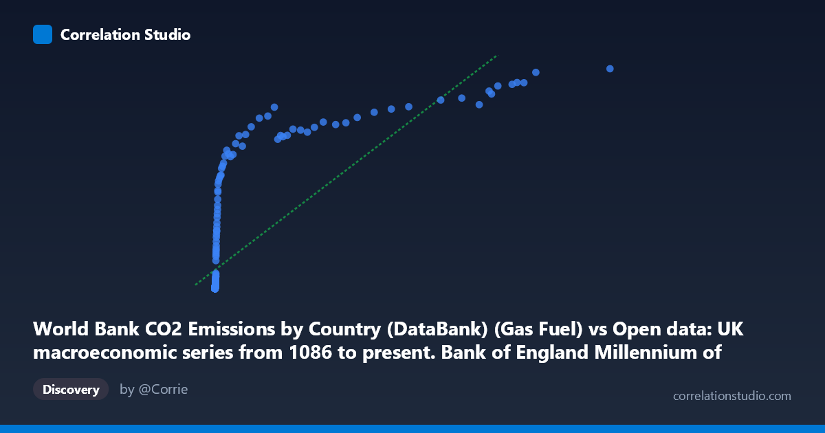
World Bank CO2 Emissions by Country (DataBank) (Gas Fuel) vs Open data: UK macroeconomic series from 1086 to present. Bank of England Millennium of Macroeconomic Data. (Month) (value)
- Pearson correlation (r)
- 0.7735
- Spearman correlation
- 0.9228
- p-value
- 0
- Sample size (n)
- 267
- 95% confidence interval
- 0.7203 to 0.8176
- Granger causality
- Bidirectional
- Granger optimal lag
- 10
AI analysis
Analysis: UK Macroeconomic Value vs. World Bank CO₂ Gas Fuel Emissions
1. Overall Relationship
The scatterplot reveals a positive but clearly non-linear relationship between World Bank CO₂ gas fuel emissions (X) and a UK macroeconomic series value (Y). At low X values (roughly below 500), points cluster near zero on the Y-axis with high density, while as X increases, Y rises steeply but then appears to plateau or compress toward an upper ceiling — suggesting a logarithmic or saturation-type curve rather than a linear one. The fitted linear regression (y = 0.187x + 1363.29) captures the general trend but visibly underfits this curvature, with the intercept of ~1363 already implying a systematic offset that linear framing struggles to explain.
2. Correlation Strength, Direction, and Causality
The Pearson r of 0.7735 indicates a moderately strong positive correlation, with r² = 0.5983 meaning approximately 60% of variance in the UK macroeconomic variable is statistically explained by gas fuel CO₂ emissions — a substantial but incomplete share, leaving 40% attributable to other factors. The 95% confidence interval of [0.7203, 0.8176] is relatively tight given n = 267, and the p-value of essentially zero confirms this association is not a sampling artifact. Crucially, Granger causality runs in both directions (X→Y: F=2.11, p=0.025; Y→X: F=2.46, p=0.008) with an optimal lag of 10 periods, suggesting a feedback loop — UK macroeconomic activity temporally predicts emissions, and emissions (or their correlated drivers) temporally predict the macroeconomic series. Neither variable is cleanly "exogenous," complicating causal interpretation. Notably, the Spearman ρ exceeds Pearson r, confirming that rank-order relationships are tighter than linear ones — a strong signal that a logarithmic or power-law model would better describe this data.
3. Notable Patterns, Clusters, and Outliers
Several structural features stand out: - Dense low-X cluster: A large mass of points sits at X < 500 with Y near zero, likely corresponding to early historical periods (pre-industrialization, 1751–early 1800s) when both emissions and UK economic output were minimal. - Upper-right saturation: Extreme X values (e.g., 116,836 → Y ≈ 15,999; 47,087 → Y ≈ 12,832) suggest Y approaches an effective ceiling around 12,000–16,000, consistent with logarithmic diminishing returns. - Notable outlier: The point (116,836, 15,999) is the most extreme on both axes and could be a high-leverage point inflating the linear r². - Mid-range scatter: Points in the X = 1,000–30,000 range show considerable vertical scatter (e.g., (2,962, 9,641) vs. (481, 4,247)), indicating significant unexplained variance in the economically active period.
4. Confounding Factors and Caveats
Several important caveats apply. First, both variables are time series spanning 1751–2017, so much of the observed correlation likely reflects a shared upward secular trend (industrialization, population growth, economic modernization) rather than a direct causal mechanism — this is a classic spurious trend correlation risk. Second, the dataset axis labels appear swapped or misattributed: the X-axis is labeled as CO₂ gas fuel emissions from the World Bank dataset but drawn from a Bank of England macroeconomic file, and vice versa for Y — this ambiguity in provenance demands careful verification before drawing conclusions. Third, the N = 18,769 population vs. n = 267 sample raises questions about how paired observations were constructed across annual vs. monthly data. Finally, bidirectional Granger causality at a 10-period lag is suggestive but does not rule out a common driver (e.g., energy price shocks, war, industrial policy) causing both variables to move together with similar lags.
5. Actionable Insights and Further Investigation
- Apply a logarithmic or power-law regression (log(X) ~ Y or Y ~ Xᵅ) to better capture the saturation curve; Spearman's advantage over Pearson strongly warrants this. - Detrend both time series (e.g., first-differencing or HP filter) before re-running Granger causality to eliminate spurious trend-driven correlations and test whether the relationship persists in cyclical components. - Segment the analysis by era (pre-1850, 1850–1950, post-1950) to determine whether the correlation structure is stable or driven by a specific industrialization phase. - Verify dataset axis provenance — the cross-labeled sources suggest a potential data join error that could materially affect interpretation. - Introduce control variables (UK population, energy prices, GDP deflator) in a multivariate framework to isolate whether emissions independently predict the macroeconomic series or merely proxy for broader economic scale.
X dataset: Open data: UK macroeconomic series from 1086 to present. Bank of England Millennium of Macroeconomic Data. (Month)
Y dataset: World Bank CO2 Emissions by Country (DataBank)
Part of experiment: Yearly - Open data: UK macroeconomic series from 1086 to present. Bank of England Millennium of Macroeconomic Data. (Month) vs World Bank CO2 Emissions by Country (DataBank)