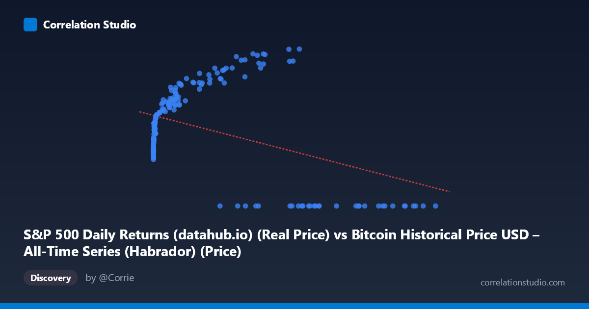
S&P 500 Daily Returns (datahub.io) (Real Price) vs Bitcoin Historical Price USD – All-Time Series (Habrador) (Price)
- Pearson correlation (r)
- -0.4161
- Spearman correlation
- 0.1073
- p-value
- 0
- Sample size (n)
- 189
- 95% confidence interval
- -0.5275 to -0.2906
- Granger causality
- None
- Granger optimal lag
- 10
- Time coverage
- 2010-08-01 to 2026-04-01
- Recomputed on refreshed data
- 2026-10-20 (r was -0.4161)
AI analysis
Analysis: Bitcoin Price vs. S&P 500 Price Relationship
1. What the Visualization Reveals
The scatterplot shows a distinctly non-linear, non-monotonic relationship despite the linear regression forcing a downward-sloping line through it. Looking at the data, low Bitcoin/X values (under ~1,000) correspond to a wide range of Y values (roughly 1,570–3,300), rising steeply as X increases from near-zero into the hundreds/thousands range. Then, at high X values (above ~30,000), Y either climbs further (into the 4,000–5,100 range) or collapses to exactly 0.00. This bimodal split at the high end — some high-X points showing Y≈0 and others showing Y≈4,500–5,100 — is the dominant visual feature and strongly suggests the "0" values represent missing or unrecorded data rather than a genuine price of zero.
2. Strength, Direction, and Statistical Confidence
The reported correlation (r = -0.416, r² = 0.173) indicates a weak-to-moderate negative linear association, but the r² tells the real story: only 17.3% of the variance in Y is explained by X, leaving over 82% unexplained by this simple linear model. The 95% CI [-0.528, -0.291] is reasonably tight and excludes zero, and the p-value (2.6×10⁻⁹) confirms this negative correlation is statistically significant and not due to chance. However, statistical significance with such large N (1,865) does not imply practical/economic significance — a modest r² means the linear relationship has limited predictive power. Critically, the Granger causality tests show no significant predictive direction in either direction (X→Y: p=0.167; Y→X: p=0.065, only marginally close to conventional thresholds). This means neither series reliably predicts future movements in the other temporally — the correlation is likely contemporaneous/coincidental or driven by a shared underlying trend rather than genuine causal lead-lag dynamics.
3. Notable Patterns and Outliers
The most striking pattern is the cluster of ~15+ points with Y = 0.00 at high X values (35,000–118,670) — this is almost certainly a data artifact (missing S&P records, delisted period, or a coding placeholder) rather than a real signal, and it's likely dragging the linear regression's negative slope. Excluding these zero-points, the "real" relationship between X and Y appears strongly positive at low-to-mid X (Y rises from ~1,570 to ~5,100 as X increases from 0 to 60,000), which contradicts the overall negative r² — a classic case of Simpson's paradox or a non-linear (possibly logarithmic or S-curve) relationship being poorly fit by a straight line. There's also a saturating/logarithmic shape at low X: Y rises very quickly from X≈0 to X≈1,000, then more gradually.
4. Confounding Factors and Caveats
Several major caveats apply. First, both series are financial time series and are likely non-stationary (trending), which can produce spurious correlations unrelated to any real economic link — differencing or using returns rather than levels would be more appropriate. Second, the zero-value cluster needs investigation; if these are missing-data codes, they should be excluded or imputed, as they materially distort both the correlation and regression fit. Third, the mismatched column descriptions (X labeled as "S&P 500 Returns" but described as Bitcoin price history, and vice versa for Y) suggest a possible data-labeling error in the source files that should be resolved before drawing economic conclusions. Finally, macroeconomic confounders (interest rates, dollar strength, crypto-specific regulatory events) likely drive both series independently, inflating apparent correlation without direct causal linkage.
5. Actionable Insights and Next Steps
Before treating this correlation as meaningful, (a) verify and clean the dataset — confirm what the Y=0 values represent and treat them as missing rather than true zeros, and correct any axis/label mismatches; (b) re-run the analysis on log-transformed or return-based (percent change) series rather than raw price levels, since both prices are likely non-stationary and this could reveal a very different (and possibly positive) relationship; (c) given the non-significant Granger results, avoid using one series to forecast the other in a trading or allocation strategy; (d) consider a non-linear or piecewise regression given the visual saturation pattern at low X; and (e) investigate common macro drivers (e.g., real interest rates, USD index) as potential confounders explaining co-movement in both assets.
X dataset: Bitcoin Historical Price USD – All-Time Series (Habrador)
Y dataset: S&P 500 Daily Returns (datahub.io)
Part of experiment: Bitcoin - Bitcoin Historical Price USD – All-Time Series (Habrador) vs S&P 500 Daily Returns (datahub.io)