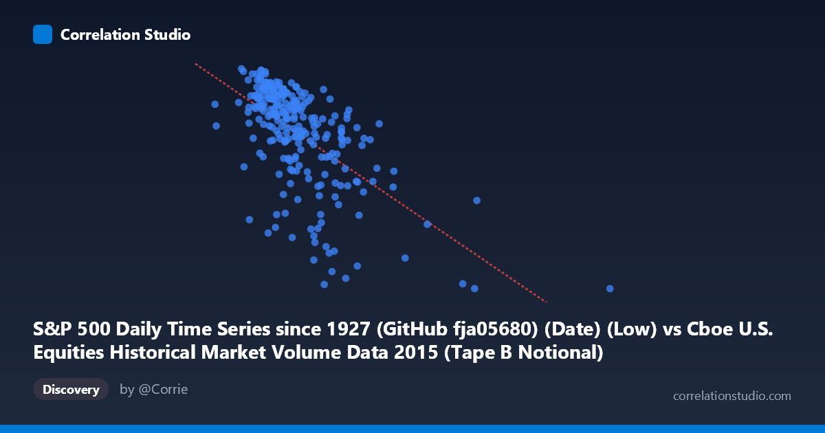
S&P 500 Daily Time Series since 1927 (GitHub fja05680) (Date) (Low) vs Cboe U.S. Equities Historical Market Volume Data 2015 (Tape B Notional)
- Pearson correlation (r)
- -0.6019
- Spearman correlation
- -0.6138
- p-value
- 0
- Sample size (n)
- 252
- 95% confidence interval
- -0.6752 to -0.5167
- Granger causality
- X → Y
- Granger optimal lag
- 7
AI analysis
Analysis: S&P 500 Daily Low vs. Cboe Tape B Notional Volume (2015)
Relationship Overview
The scatterplot reveals a negative relationship between the S&P 500 daily low price (X-axis) and Cboe Tape B notional trading volume (Y-axis) across 252 trading days in 2015. As the S&P 500's daily low increases, Tape B notional volume tends to decrease. This is an intuitively meaningful pattern: higher index price levels are generally associated with calmer, lower-volatility market conditions that attract less urgent trading activity, while lower price levels — often coinciding with market stress or corrections — tend to drive elevated notional volumes as participants react to adverse moves.
Correlation Strength and Statistical Significance
The Pearson correlation of r = -0.60 indicates a moderate-to-strong negative association. The R² of 0.362 means that roughly 36% of the variance in Tape B notional volume is explained by the S&P 500 daily low, leaving approximately 64% attributable to other factors. The 95% confidence interval of [-0.675, -0.517] is meaningfully narrow and sits entirely in negative territory, confirming the direction is not a statistical artifact. The p-value of effectively zero (against a population of N = 3,302) makes the relationship highly significant. Critically, the Granger causality analysis identifies a unidirectional temporal relationship: X Granger-causes Y at an optimal lag of 7 trading periods (F = 2.20, p = 0.035), while the reverse direction fails to reach significance (F = 0.83, p = 0.56). This suggests that S&P 500 price levels carry predictive information about future Tape B notional volume approximately 1–1.5 weeks ahead, not merely a contemporaneous coincidence.
Notable Patterns, Clusters, and Outliers
The data exhibits a visible clustering structure rather than a smooth linear band. A dense cluster of observations occupies the X range of roughly 3.5–6.5 billion (index low range approximately 2,040–2,126), forming a relatively tight core. Beyond ~7 billion on the X-axis, the relationship becomes sparser and more dispersed, with several notable outliers at extreme X values (e.g., points near 12.5 billion with Y values as low as ~1,867–1,971). These high-X, low-Y outliers likely correspond to August 2015 market volatility — when the S&P 500 suffered a sharp correction — driving anomalously high notional volumes at depressed price levels. The linear regression line (y = -2.007×10⁻⁸x + 2158.87) appears to fit the central cluster reasonably, but likely underestimates the curvature at extremes.
Confounding Factors and Caveats
Several important caveats apply. First, Tape B specifically covers NYSE American (AMEX) and regional exchange listings, making it a partial, not comprehensive, measure of market volume — its dynamics may differ from total market notional. Second, the S&P 500 daily low is inherently a stress-sensitive metric (it captures intraday downside), potentially amplifying the negative relationship with volume compared to using closing prices. Third, time-series autocorrelation is almost certainly present in both variables (prices trend, volume clusters), which can inflate apparent correlation and complicate inference. The Granger result, while suggestive, does not imply economic causation — both variables may respond to a common driver such as the VIX (volatility index), macroeconomic news, or Federal Reserve communications. The August 2015 flash crash period likely exerts disproportionate leverage on the regression coefficients.
Actionable Insights and Further Investigation
The 7-day Granger lag is an operationally interesting finding worth investigating further: it raises the question of whether declining S&P 500 price levels systematically precede elevated Tape B activity by approximately a week, possibly reflecting delayed institutional repositioning or options-related hedging flows. Recommended next steps include: (1) adding VIX as a control variable to test whether the S&P–volume relationship survives after accounting for explicit volatility expectations; (2) segmenting the analysis by market regime (e.g., pre- and post-August correction) to assess structural stability; (3) examining Tape A and C volumes to determine whether the relationship is Tape B-specific or market-wide; and (4) testing non-linear models (e.g., piecewise regression or GAM) given the apparent threshold behavior at higher X values. The 36% explained variance suggests a genuinely informative signal worth refining rather than dismissing.
X dataset: Cboe U.S. Equities Historical Market Volume Data 2015
Y dataset: S&P 500 Daily Time Series since 1927 (GitHub fja05680) (Date)
Part of experiment: Daily - Cboe U.S. Equities Historical Market Volume Data 2015 vs S&P 500 Daily Time Series since 1927 (GitHub fja05680) (Date)