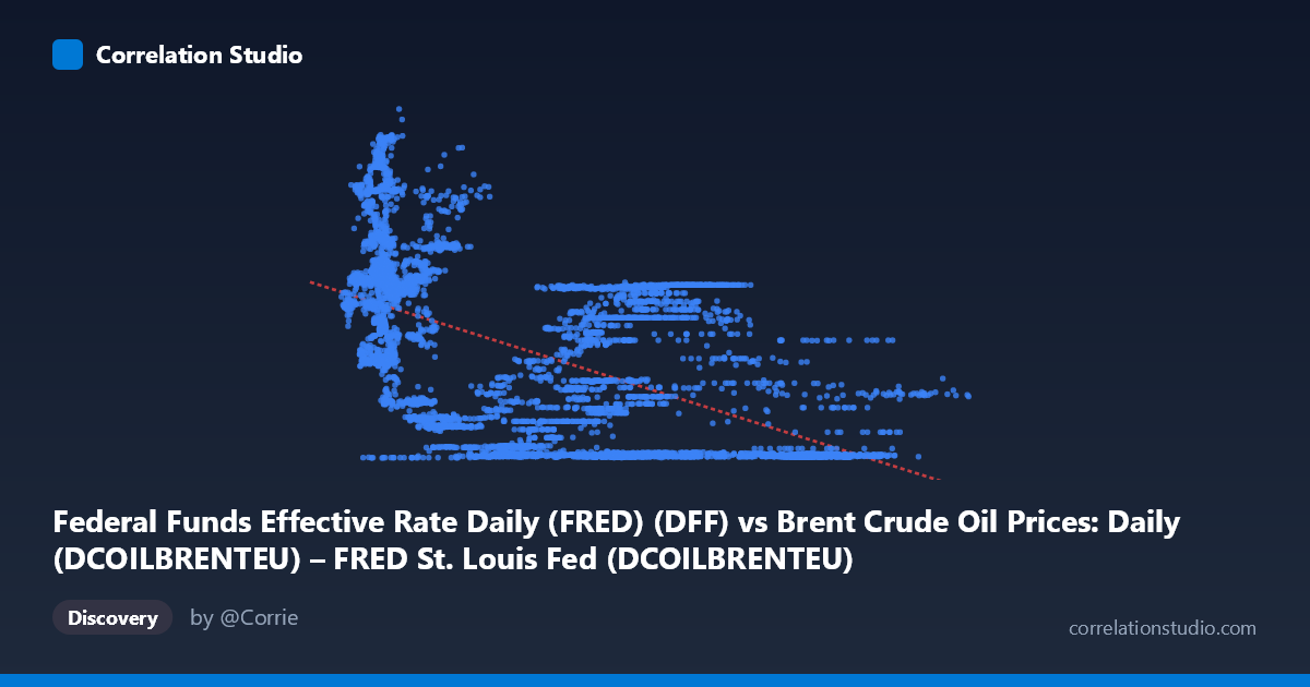
Federal Funds Effective Rate Daily (FRED) (DFF) vs Brent Crude Oil Prices: Daily (DCOILBRENTEU) – FRED St. Louis Fed (DCOILBRENTEU)
- Pearson correlation (r)
- -0.5438
- Spearman correlation
- -0.5951
- p-value
- 0
- Sample size (n)
- 9893
- 95% confidence interval
- -0.5576 to -0.5298
- Granger causality
- None
- Granger optimal lag
- 1
AI analysis
Federal Funds Rate vs. Brent Crude Oil Price: Correlation Analysis
Overall Relationship
The scatterplot reveals a negative, moderately weak relationship between the Federal Funds Effective Rate (X-axis) and Brent Crude Oil prices (Y-axis), described by the linear regression equation y = -0.04485x + 5.526. At first glance, this suggests that higher interest rates are associated with lower oil prices — a relationship that carries some intuitive economic logic, as tighter monetary policy can suppress demand and strengthen the dollar, both of which tend to weigh on commodity prices. However, the visualization also clearly shows substantial scatter, non-linearity, and distinct clustering patterns that caution against over-interpreting any simple linear narrative.
Correlation Strength and Statistical Significance
The Pearson correlation of r = -0.544 indicates a moderate negative association, but the R² of 0.296 means that only about 29.6% of the variance in oil prices is explained by the federal funds rate — leaving over 70% of variation attributable to other factors. The 95% confidence interval for r is tight ([-0.558, -0.530]), which reflects the large paired sample size (n = 9,893) rather than a particularly precise underlying relationship; with nearly 10,000 observations, even modest correlations achieve high statistical certainty. The p-value of effectively zero confirms the result is not due to chance. Critically, however, Granger causality tests find no significant predictive directionality in either direction — neither does the Fed rate predict future oil prices (F = 0.976, p = 0.323), nor do oil prices predict future Fed rates (F = 0.115, p = 0.734). This is a pivotal finding: the correlation is statistically real, but neither variable appears to temporally drive the other at the tested lag, strongly implying the relationship is driven by shared confounders or long-run structural co-movement rather than direct causation.
Notable Patterns, Clusters, and Non-Linearity
Several distinct features stand out in the data:
- High-rate, low-oil cluster: Points with X values above ~70–80 (high Fed funds rate) cluster heavily near Y values of 0.1–0.5, reflecting the early-to-mid 1980s era when Volcker-era rates were extreme and oil prices had collapsed from their 1980 peak. - Low-rate, variable-oil dispersion: At low X values (Fed rate near 0–20), oil prices span nearly the full Y range (roughly 1 to 10+), indicating that low interest rate environments correspond to highly variable oil prices — from post-2008 near-zero rate periods with both high and low oil, to COVID-era collapses. - Curved, hyperbolic-like shape: The relationship is visibly non-linear. Oil prices decay sharply as rates rise from 0 to ~50, then flatten near zero for rates above 70–80, suggesting a diminishing marginal effect or a structural regime break rather than a linear process. - Outliers: Several sample points show high oil values (Y 7–8) at low-to-moderate X values (e.g., 13.20, 8.21; 15.63, 3.70; 16.53, 8.24), likely corresponding to 2005–2008 oil price spikes during a period of gradually rising rates.
Confounding Factors and Caveats
This correlation almost certainly reflects spurious co-movement driven by historical macroeconomic regimes rather than a direct causal mechanism. Both variables are shaped powerfully by the same underlying forces: global recessions (2008, 2020), geopolitical shocks (Gulf Wars, OPEC supply decisions, Ukraine conflict), and long structural shifts in U.S. monetary policy cycles. The axis labels appear to be swapped in the dataset metadata (DFF is described under the Brent dataset and vice versa), which should be verified before drawing firm conclusions. Additionally, the time coverage spanning 1987–2026 encompasses radically different monetary and oil market regimes (Volcker disinflation, dot-com era, zero lower bound, post-COVID inflation), making the pooled correlation a blend of structurally distinct periods. A single linear model across nearly four decades is likely masking substantial regime-dependent heterogeneity.
Actionable Insights and Further Investigation
Given these findings, several next steps are warranted:
1. Segment by monetary regime: Split the data into distinct Fed policy eras (high-rate 1987–1995, moderate 1995–2008, near-zero 2008–2015, normalization 2015–2019, COVID/post-COVID 2020–present) and compute within-regime correlations separately. 2. Test non-linear models: Fit a logarithmic or power-law regression (e.g., log(Y) ~ X), which would likely improve R² substantially given the apparent hyperbolic shape. 3. Include mediating variables: Oil demand proxies (global GDP growth, industrial production), OPEC supply decisions, and USD index should be included in a multivariate model to isolate any independent Fed rate effect. 4. Extend Granger tests to longer lags: The absence of Granger causality at lag 1 (daily) does not rule out predictive relationships at monthly or quarterly lags, which are more relevant to monetary transmission. 5. Verify data alignment: Confirm that Fed funds rate and Brent price series are properly date-aligned, especially given the metadata label swap noted above, to ensure paired observations are economically meaningful.
X dataset: Brent Crude Oil Prices: Daily (DCOILBRENTEU) – FRED St. Louis Fed
Y dataset: Federal Funds Effective Rate Daily (FRED)
Part of experiment: Daily - Brent Crude Oil Prices: Daily (DCOILBRENTEU) – FRED St. Louis Fed vs Federal Funds Effective Rate Daily (FRED)