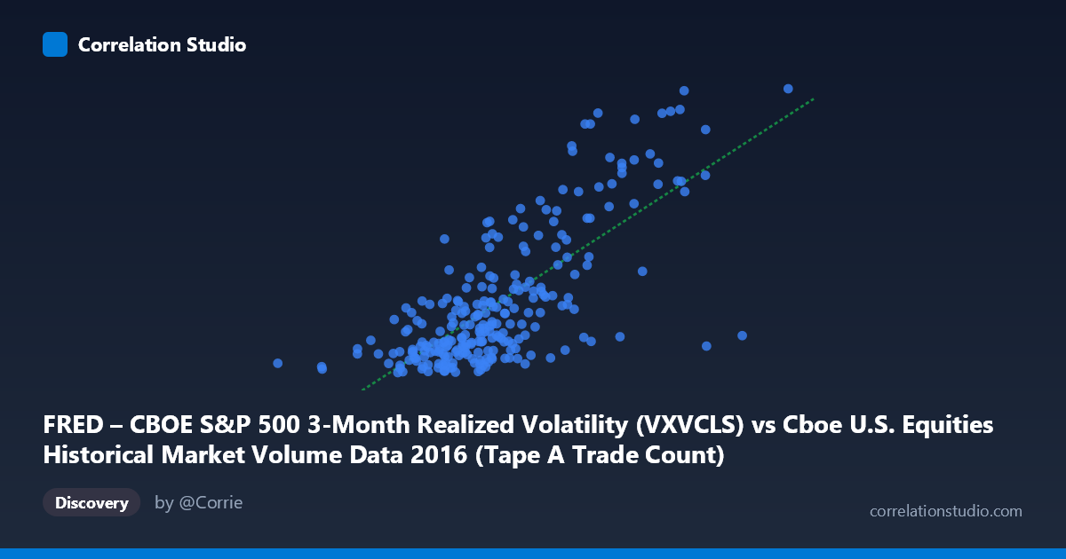
FRED – CBOE S&P 500 3-Month Realized Volatility (VXVCLS) vs Cboe U.S. Equities Historical Market Volume Data 2016 (Tape A Trade Count)
- Pearson correlation (r)
- 0.7384
- Spearman correlation
- 0.6797
- p-value
- 0
- Sample size (n)
- 252
- 95% confidence interval
- 0.6765 to 0.7899
- Granger causality
- None
- Granger optimal lag
- 1
AI analysis
Analysis: CBOE S&P 500 3-Month Realized Volatility vs. Tape A Trade Count (2016)
Relationship Overview The scatterplot reveals a moderately strong positive relationship between CBOE S&P 500 3-month realized volatility (VXVCLS) and Tape A trade counts on U.S. equity exchanges throughout 2016. As volatility rises, trade counts increase in a broadly consistent manner, which aligns with intuitive market dynamics: periods of elevated uncertainty tend to drive higher trading activity as market participants reposition, hedge, or react to price movements. The linear regression equation (y = 7.54×10⁻⁶x + 7.78) suggests that each unit increase in the volatility index corresponds to a measurable — though modest in absolute terms — uptick in trade counts.
Correlation Strength and Statistical Significance The correlation coefficient of r = 0.7384 indicates a meaningful positive association, and the R² of 0.5452 tells us that approximately 54.5% of the variance in Tape A trade counts is explained by the VXVCLS volatility index — a substantial but incomplete picture, leaving ~45.5% of variance attributable to other factors. The 95% confidence interval for r [0.6765, 0.7899] is relatively tight and does not approach zero, lending credibility to the finding, while the p-value of effectively 0 (with n = 252 paired observations drawn from a population of 3,622) confirms the relationship is highly unlikely to be a statistical artifact. However, the Granger causality results are notably absent of significance in either direction (X→Y: F = 1.13, p = 0.289; Y→X: F = 0.19, p = 0.666). This is a critical caveat: despite a strong contemporaneous correlation, neither variable significantly predicts the other temporally at a 1-period lag. This means the relationship is likely coincident rather than causal — both variables may be responding simultaneously to the same underlying market conditions rather than one driving the other.
Notable Patterns and Outliers The sample points reveal several important structural features. The bulk of observations cluster in the lower-left region of the scatterplot — volatility readings between roughly 1,000,000–1,500,000 and trade counts between 15–19 — suggesting that 2016 was predominantly a low-to-moderate volatility year. However, there are clear high-leverage outliers in the upper-right region, with points such as (2,013,606, 26.71) and (1,860,056, 24.02) representing spikes likely associated with identifiable market events (e.g., Brexit vote in June 2016, U.S. election in November 2016). These outliers are disproportionately influential on the regression slope and correlation coefficient. There is also a hint of non-linearity or heteroscedasticity: variance in trade counts appears to widen at higher volatility levels, suggesting the relationship may not be strictly linear across all regimes.
Confounding Factors and Caveats Several confounding factors warrant caution. First, 2016 was not a typical year — it contained the Brexit referendum and a U.S. presidential election, both of which simultaneously spiked volatility and trading volumes, making it difficult to disentangle structural relationships from event-driven co-movement. Second, the axes may be swapped in dataset labeling (X-axis is described as VXVCLS but sourced from the volume dataset, and vice versa for Y), which should be verified before drawing firm conclusions. Third, trade counts are influenced by factors entirely independent of volatility — algorithmic trading schedules, end-of-quarter rebalancing, market microstructure changes, and exchange rule changes — none of which are captured here. Finally, the 1-period lag used in Granger testing may be too short to detect meaningful predictive relationships, and testing across multiple lags could yield different conclusions.
Actionable Insights and Further Investigation Practitioners should treat this correlation as a useful risk-monitoring signal rather than a predictive tool: when implied/realized volatility spikes, expect elevated trade volumes and plan infrastructure, liquidity management, and execution strategies accordingly. For further investigation, it would be valuable to (1) extend the Granger causality analysis to 3–10 lag periods to rule out delayed predictive dynamics; (2) disaggregate by event type (e.g., remove Brexit and election days) to test whether the correlation holds in calmer regimes; (3) test non-linear models (e.g., log-log or piecewise regression) given the apparent heteroscedasticity; and (4) introduce control variables such as VIX term structure, macro news release calendars, or index futures open interest to better isolate the direct volatility-to-volume mechanism.
X dataset: Cboe U.S. Equities Historical Market Volume Data 2016
Y dataset: FRED – CBOE S&P 500 3-Month Realized Volatility
Part of experiment: Daily - Cboe U.S. Equities Historical Market Volume Data 2016 vs FRED – CBOE S&P 500 3-Month Realized Volatility