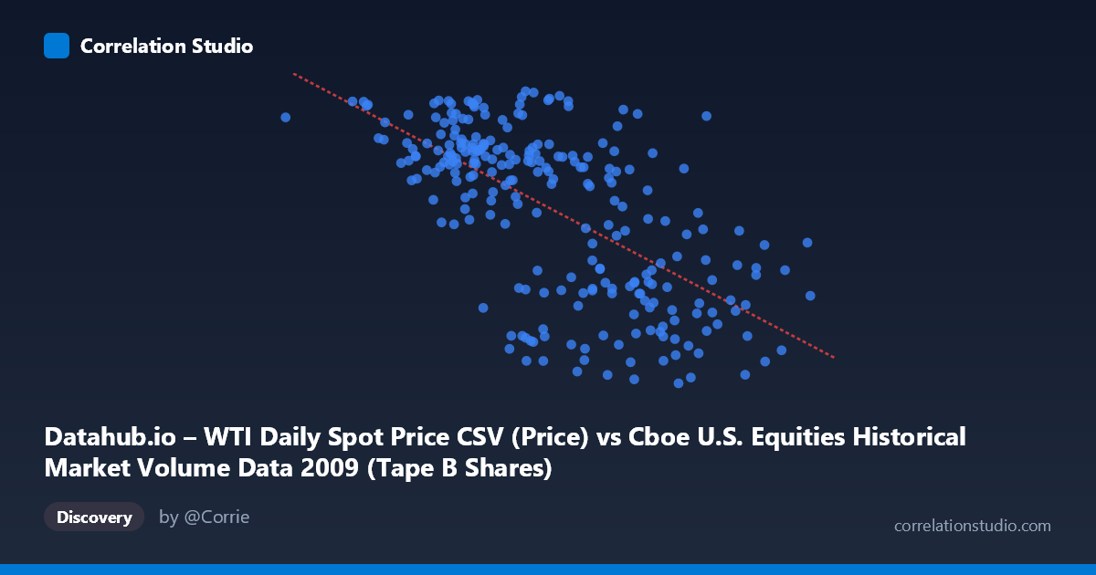
Datahub.io – WTI Daily Spot Price CSV (Price) vs Cboe U.S. Equities Historical Market Volume Data 2009 (Tape B Shares)
- Pearson correlation (r)
- -0.6387
- Spearman correlation
- -0.6337
- p-value
- 0
- Sample size (n)
- 252
- 95% confidence interval
- -0.7065 to -0.5593
- Granger causality
- None
- Granger optimal lag
- 1
AI analysis
Scatterplot Analysis: WTI Oil Price vs. Cboe Tape B Share Volume (2009)
Relationship Overview The scatterplot reveals a moderate negative relationship between WTI daily spot oil prices (X-axis) and Cboe Tape B share volumes (Y-axis) across 252 trading days in 2009. The linear regression equation (y = -1.999×10⁻⁷x + 91.30) confirms that as oil prices rise, Tape B equity share volumes tend to decline. This pattern is visually apparent in the data: lower X values (cheaper oil, roughly $33–$100/barrel range) cluster toward higher Y values (greater share volumes, 70–81), while higher X values (more expensive oil, $175–$255 range) tend to associate with lower share volumes (35–55). The relationship, while real, shows considerable scatter, suggesting the story is more complex than a simple linear dynamic.
Correlation Strength and Statistical Significance The Pearson correlation of r = -0.6387 indicates a moderate-to-strong negative association. The r² = 0.4079 is the critical interpretive figure here — roughly 40.8% of the variance in Tape B share volumes is explained by WTI oil prices, meaning nearly 60% of variance remains unexplained by this model alone. The 95% confidence interval of [-0.7065, -0.5593] is meaningfully narrow and entirely negative, providing strong statistical confidence that the true population correlation is genuinely negative and non-trivial. The p-value of essentially zero (given N = 3,232 underlying observations and n = 252 paired samples) confirms this is highly unlikely to be a chance finding. However, the Granger causality results are striking in their absence: neither direction (X→Y: F = 0.0020, p = 0.9642; Y→X: F = 1.1867, p = 0.2771) shows statistically significant temporal predictive power. This means that while the two variables co-move, neither one leads the other in a forecasting sense — the correlation is contemporaneous and associative, not directionally causal at lag-1.
Notable Patterns, Clusters, and Outliers Several structural features emerge from the sample points. There is a distinct high-volume cluster concentrated at lower oil prices (X ≈ $65M–$130M range, corresponding to roughly $65–$130/barrel), where Tape B volumes consistently range from 67 to 81 — suggesting a floor or natural trading range for shares. Conversely, the high-price, low-volume region (X $175M) shows more compressed volume values (35–58) with less variability. The point at (33,822,027, 76.83) stands out as an extreme low-price outlier — likely representing early 2009 when oil was near its post-crisis nadir — and it aligns with high volume, consistent with the overall trend. The point at (254,504,132, 56.67) anchors the upper-right, reflecting late-year price recovery. Notably, the scatter is heteroscedastic: variance in Y appears larger at mid-range X values, narrowing at extremes, which weakly violates linear regression assumptions.
Confounding Factors and Interpretive Caveats The year 2009 was extraordinary — the global financial crisis recovery, TARP effects, quantitative easing, and sector-specific volatility all independently drove both oil prices and equity volumes. Oil prices nearly tripled from roughly $33 to $81/barrel during this single year, largely reflecting macroeconomic recovery rather than supply/demand fundamentals alone. This means the correlation may be capturing a shared recovery trajectory rather than a direct mechanism: as the economy recovered, oil prices rose while equity market structure evolved (high-frequency trading, institutional deleveraging) potentially suppressing Tape B volumes. The Tape B designation (primarily NYSE Arca-listed securities, including many energy ETFs) adds a sector composition layer — oil price changes may directly affect the valuation and thus trading interest in the underlying securities. The absence of Granger causality further cautions against assuming that oil prices drive volume decisions, or vice versa.
Actionable Insights and Further Investigation The moderate correlation and absent Granger causality together suggest that both variables are likely co-driven by a common underlying factor — most plausibly macroeconomic sentiment or risk appetite in 2009. Investigators should consider: (1) Adding a risk sentiment proxy (e.g., VIX) as a control variable to test whether the oil-volume correlation weakens significantly after conditioning on market fear; (2) Extending the time series beyond 2009 to test whether this relationship holds in non-crisis years, or whether it is an artifact of the recovery dynamics specific to this period; (3) Testing non-linear models — the visible heteroscedasticity and the natural floor/ceiling behavior in both variables suggest a log-log or piecewise regression might substantially improve on the 40.8% explained variance; and (4) Examining lag structures beyond lag-1 in Granger testing, as weekly or monthly aggregation might reveal delayed transmission channels not visible at daily resolution.
X dataset: Cboe U.S. Equities Historical Market Volume Data 2009
Y dataset: Datahub.io – WTI Daily Spot Price CSV
Part of experiment: Daily - Cboe U.S. Equities Historical Market Volume Data 2009 vs Datahub.io – WTI Daily Spot Price CSV