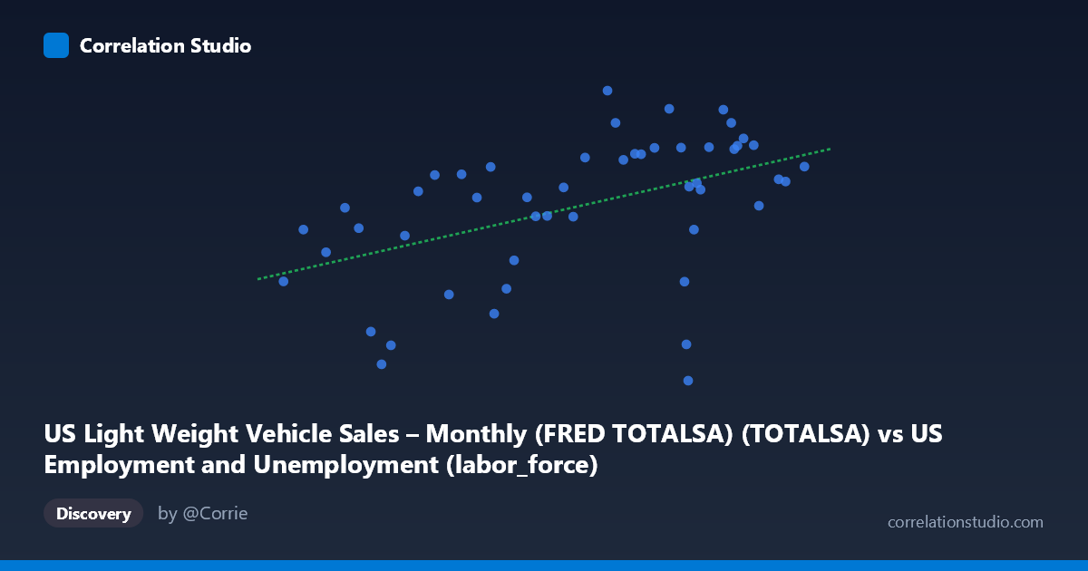
US Light Weight Vehicle Sales – Monthly (FRED TOTALSA) (TOTALSA) vs US Employment and Unemployment (labor_force)
- Pearson correlation (r)
- 0.4718
- Spearman correlation
- 0.5363
- p-value
- 0.000542
- Sample size (n)
- 50
- 95% confidence interval
- 0.2227 to 0.6631
- Granger causality
- None
- Granger optimal lag
- 1
AI analysis
Scatterplot Analysis: US Light Vehicle Sales vs. Labor Force Size
Overall Relationship The scatterplot reveals a moderate positive relationship between US light weight vehicle sales (X-axis, measured in thousands of units SAAR) and the US labor force size (Y-axis, in millions). As vehicle sales increase, labor force participation tends to rise as well. The linear regression equation y = 4.657e-05x + 8.633 confirms this upward trend, suggesting that for every increase of roughly 21,500 units in vehicle sales, the labor force grows by approximately one million workers. Visually, the data points trend upward from lower-left to upper-right, though with considerable scatter around the fitted line, indicating the relationship is real but far from deterministic.
Correlation Strength and Statistical Significance The Pearson correlation of r = 0.456 indicates a moderate positive association, but the coefficient of determination r² = 0.208 is the more telling statistic — only 20.8% of the variance in labor force size is explained by vehicle sales levels. The remaining ~79% is attributable to other factors entirely. The 95% confidence interval of [0.204, 0.652] is relatively wide, reflecting meaningful uncertainty in the true population correlation, though it does not cross zero. The p-value of 0.0009 confirms the result is statistically significant at conventional thresholds (p < 0.001), so this is unlikely a chance finding given the sample of n = 50 paired observations drawn from a population of N = 86. However, statistical significance should not be conflated with practical importance given the modest variance explained. Critically, Granger causality tests in both directions fail to reach significance (X→Y: F = 1.007, p = 0.321; Y→X: F = 0.556, p = 0.460), meaning neither variable demonstrably predicts the other in a temporal lead-lag sense at a 1-period lag. This strongly cautions against any causal interpretation.
Notable Patterns, Clusters, and Outliers Several features stand out in the point cloud. There appears to be a loose cluster of high-sales observations (X 150,000) with moderate-to-high labor force values (Y = 15–18), consistent with the general trend. However, notable outliers disrupt the pattern: the point near (154,142; 9.79) represents an anomalously low labor force value at relatively high vehicle sales — this is the most visually prominent outlier and likely reflects a data alignment or temporal mismatch issue. Similarly, (110,204; 10.29) and (111,550; 10.87) show low values on both axes, possibly reflecting recessionary periods (early 1980s or 2008–2009 era). The spread widens at higher X values, hinting at possible heteroscedasticity — variance in labor force size may increase as vehicle sales grow, which could subtly inflate correlation estimates.
Confounding Factors and Interpretive Caveats The most important caveat here is that both variables are strongly driven by shared underlying macroeconomic conditions — GDP growth, business cycles, population growth, and consumer confidence all independently influence both auto sales and labor force participation. The observed correlation almost certainly reflects common dependence on the broader economy rather than any direct mechanistic link between buying cars and labor force size. The datasets also originate from different temporal resolutions (monthly SAAR for vehicle sales vs. annual labor force data), and the 1976–2025 time coverage spans multiple structural regime changes including oil shocks, recessions, demographic shifts (Baby Boomer retirements), and COVID-19 — all of which could create spurious correlation across long time series. The Granger non-causality result reinforces that no predictive temporal structure exists between these variables at the measured lag.
Actionable Insights and Further Investigation Given the moderate correlation, limited variance explained, and absent Granger causality, practitioners should avoid using vehicle sales as a standalone predictor of labor force dynamics (or vice versa). Instead, both should be treated as co-varying economic indicators rather than causally linked variables. Recommended next steps include: (1) controlling for GDP or the unemployment rate as a shared confounder to isolate any residual relationship; (2) testing multiple Granger lags (beyond the single-period tested here) given the mixed temporal resolutions; (3) segmenting the data by era (pre/post-2008, pre/post-COVID) to check whether the correlation is stable or driven by specific economic regimes; and (4) investigating the extreme outlier at (154,142; 9.79) to determine whether it represents a data quality issue or a genuinely important historical anomaly worth contextualizing.
X dataset: US Employment and Unemployment
Y dataset: US Light Weight Vehicle Sales – Monthly (FRED TOTALSA)
Part of experiment: Yearly - US Employment and Unemployment vs US Light Weight Vehicle Sales – Monthly (FRED TOTALSA)