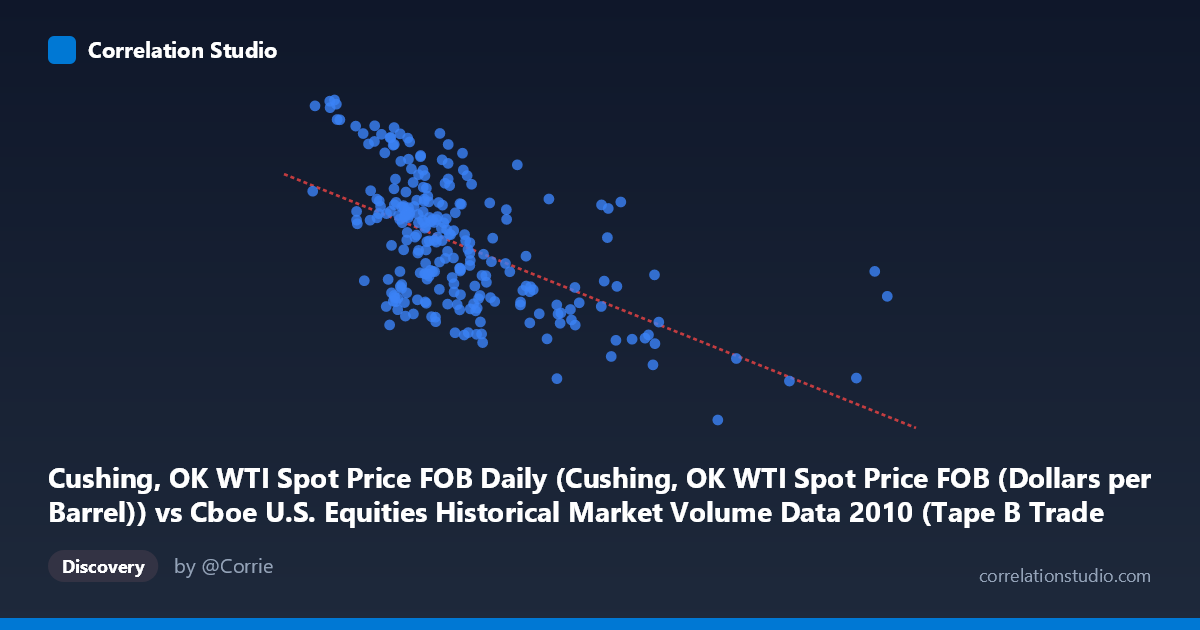
Cushing, OK WTI Spot Price FOB Daily (Cushing, OK WTI Spot Price FOB (Dollars per Barrel)) vs Cboe U.S. Equities Historical Market Volume Data 2010 (Tape B Trade Count)
- Pearson correlation (r)
- -0.5644
- Spearman correlation
- -0.55
- p-value
- 0
- Sample size (n)
- 252
- 95% confidence interval
- -0.6431 to -0.4739
- Granger causality
- None
- Granger optimal lag
- 1
AI analysis
Analysis: WTI Crude Oil Price vs. Cboe Tape B Trade Count (2010)
Relationship Overview The scatterplot reveals a moderate negative relationship between WTI crude oil spot prices (X-axis) and Cboe Tape B equity trade counts (Y-axis) across 252 trading days in 2010. As oil prices rise, equity trade counts on Tape B tend to decline, and this inverse pattern is visually evident in the downward slope of the regression line (y = -2.34×10⁻⁵x + 86.578). The relationship is discernible but not tight — data points show considerable scatter around the regression line, indicating that oil price alone is far from a complete explanation of trading activity levels.
Correlation Strength and Statistical Interpretation The Pearson correlation of r = -0.5644 reflects a moderate negative association. However, the coefficient of determination r² = 0.3186 is the more practically meaningful figure: oil prices explain only about 31.9% of the variance in Tape B trade counts, meaning roughly 68% of the variation in trading activity is attributable to other factors entirely. The 95% confidence interval of [-0.6431, -0.4739] is meaningfully narrow given the sample size of 252, and the p-value of effectively zero confirms this correlation is highly unlikely to be a sampling artifact. That said, the Granger causality tests reveal no significant temporal predictive relationship in either direction (X→Y: F=0.63, p=0.43; Y→X: F=2.50, p=0.11), which is a critical caveat — despite the cross-sectional correlation, neither variable reliably predicts the other's future values at a one-period lag. This dissociation between correlation and Granger causality strongly suggests a spurious or confounded contemporaneous relationship rather than a direct causal mechanism.
Notable Patterns, Clusters, and Outliers Several structural features stand out. At lower oil price values (roughly $150,000–$300,000 range on the x-axis, noting the x-axis appears to represent a scaled or notional price figure), trade counts span a wide range from approximately 73 to 91, indicating high variability when prices are low. At higher oil price levels (above $500,000), trade counts cluster tightly in the 64–76 range, suggesting a compression of trading activity under elevated oil price conditions. There are a handful of notable outliers: the point near (918,659, 75.10) represents an extreme high oil price observation with a near-median trade count, and points like (675,996, 64.78) and (778,565, 68.03) anchor the lower-right corner of the plot, reinforcing the negative trend. Conversely, several high-trade-count observations (88–91 range) cluster at low oil prices, including (120,757, 90.84) and (184,594, 89.33), which appear to be influential leverage points driving much of the observed correlation.
Confounding Factors and Caveats Interpreting this correlation as causal would be premature for several reasons. First, both variables are likely driven by common macroeconomic conditions — early 2010 was a post-financial-crisis recovery period where risk sentiment, Federal Reserve policy, and economic data releases simultaneously influenced commodity prices and equity market activity. Second, Tape B specifically covers NYSE American (AMEX) and regional exchange-listed securities, a niche segment whose volume dynamics may be more sensitive to specific market microstructure changes (e.g., routing rule changes, maker-taker fee adjustments) than to oil prices per se. Third, the x-axis values appear unusually large for a per-barrel oil price (WTI traded in the $70–$92 range in 2010), suggesting the variable may represent a notional value or volume-weighted price construct rather than a simple spot price, which complicates direct interpretation. The failure of Granger causality tests further underscores that this correlation is likely contemporaneous and driven by shared latent drivers rather than any direct oil-price-to-trading-activity mechanism.
Actionable Insights and Further Investigation Given these findings, several investigative paths are warranted. First, introduce macroeconomic control variables — VIX (volatility index), S&P 500 returns, and Federal Reserve policy announcements — to test whether the oil-trade-count correlation survives adjustment for broader market conditions. Second, examine the x-axis variable definition carefully: if it represents notional traded value rather than spot price, the correlation may actually reflect a joint volume effect (high-volume days see both large notional oil values and high equity trade counts, or vice versa), which would be a fundamentally different story. Third, testing longer lag structures in Granger causality (beyond the optimal 1-period lag tested here) might reveal delayed transmission channels. Finally, segmenting the data by market regime (e.g., low vs. high volatility periods, pre- and post-May 2010 Flash Crash) could reveal whether the negative relationship is consistent throughout 2010 or driven by specific episodic windows.
X dataset: Cboe U.S. Equities Historical Market Volume Data 2010
Y dataset: Cushing, OK WTI Spot Price FOB Daily
Part of experiment: Daily - Cboe U.S. Equities Historical Market Volume Data 2010 vs Cushing, OK WTI Spot Price FOB Daily