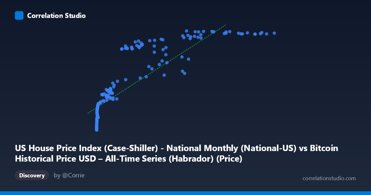
US House Price Index (Case-Shiller) - National Monthly (National-US) vs Bitcoin Historical Price USD – All-Time Series (Habrador) (Price)
- Pearson correlation (r)
- 0.8512
- Spearman correlation
- 0.9698
- p-value
- 0
- Sample size (n)
- 189
- 95% confidence interval
- 0.8065 to 0.8863
- Granger causality
- None
- Granger optimal lag
- 9
AI analysis
Analysis: Bitcoin Price vs. US Case-Shiller Home Price Index
1. What the Visualization Reveals
The scatterplot shows a strong positive association between Bitcoin's historical USD price (X-axis) and the US Case-Shiller National Home Price Index (Y-axis). However, the relationship is clearly non-linear: at low Bitcoin prices (roughly $0–$1,000), the Case-Shiller index climbs steeply from ~137 to ~190, then the curve flattens considerably as Bitcoin prices rise into the tens of thousands, with the index compressing into a narrower band (roughly 240–330). This produces a logarithmic or saturating-curve shape rather than a straight line — consistent with the note that Spearman's ρ exceeds Pearson's r.
2. Strength, Direction, and Statistical Confidence
The Pearson correlation (r = 0.847) is strong and positive, with r² = 0.717 indicating that a linear model explains about 72% of the variance in the housing index from Bitcoin price alone — a substantial share, though nearly 28% remains unexplained by this simple relationship. The 95% CI [0.801, 0.883] is tight and the p-value is essentially 0, confirming this correlation is highly unlikely to be a sampling artifact given n=187. Critically, however, the Granger causality tests show no significant predictive direction in either direction (X→Y: p=0.30; Y→X: p=0.12). This means that despite the strong contemporaneous correlation, neither variable's past values reliably help forecast the other's future values at a 1-period lag — the relationship is likely driven by a shared external trend (e.g., both being driven by time/macroeconomic conditions) rather than one causing the other.
3. Notable Patterns and Outliers
- Two-regime structure: A steep, near-vertical rise for X < $1,000 (Bitcoin's early years, 2010–2013) transitions into a much flatter, saturating relationship at higher prices — suggesting log(X) would fit far better than raw X. - Compression at high X: Once Bitcoin exceeds ~$50,000, Y values cluster tightly between 300–330, implying the housing index has its own ceiling/growth ceiling largely independent of further Bitcoin appreciation. - Some scatter/noise at mid-range X (e.g., $29,000–$58,000 shows Y values swinging from 239 to 320), indicating other factors modulate Y independent of Bitcoin price during this era. - No extreme outliers break the general curve shape; the data appears to trace a smooth, single monotonic path.
4. Confounding Factors and Caveats
Both series are time-indexed and non-stationary — Bitcoin price and US home prices have both trended upward over the 2010–2026 window largely due to independent macro forces (monetary policy, low interest rates, inflation, post-2020 stimulus, crypto adoption cycles). This is a classic case where time itself is the lurking confounder: correlating two upward-trending time series will produce spuriously high r values even without direct causal linkage. The lack of Granger causality reinforces that this is likely a coincidental co-trending relationship rather than a genuine economic linkage. Additionally, comparing a monthly-sampled housing index to a much higher-frequency Bitcoin price series raises alignment/aggregation concerns.
5. Actionable Insights
- Detrend or difference both series (e.g., use year-over-year % changes rather than levels) before correlating, to test whether the relationship survives removing shared trend — this would give a much more honest measure of true co-movement. - Fit a log-linear model (Y vs. log(X)) given the visual and Spearman-vs-Pearson evidence of non-linearity; this will likely improve fit and interpretability. - Treat this correlation as descriptive, not causal or predictive — the Granger results explicitly rule out using one series to forecast the other. - Consider a third-variable analysis (e.g., Fed funds rate, M2 money supply, or general market risk appetite) as a common driver explaining both trends.
X dataset: Bitcoin Historical Price USD – All-Time Series (Habrador)
Y dataset: US House Price Index (Case-Shiller) - National Monthly
Part of experiment: Bitcoin - Bitcoin Historical Price USD – All-Time Series (Habrador) vs US House Price Index (Case-Shiller) - National Monthly