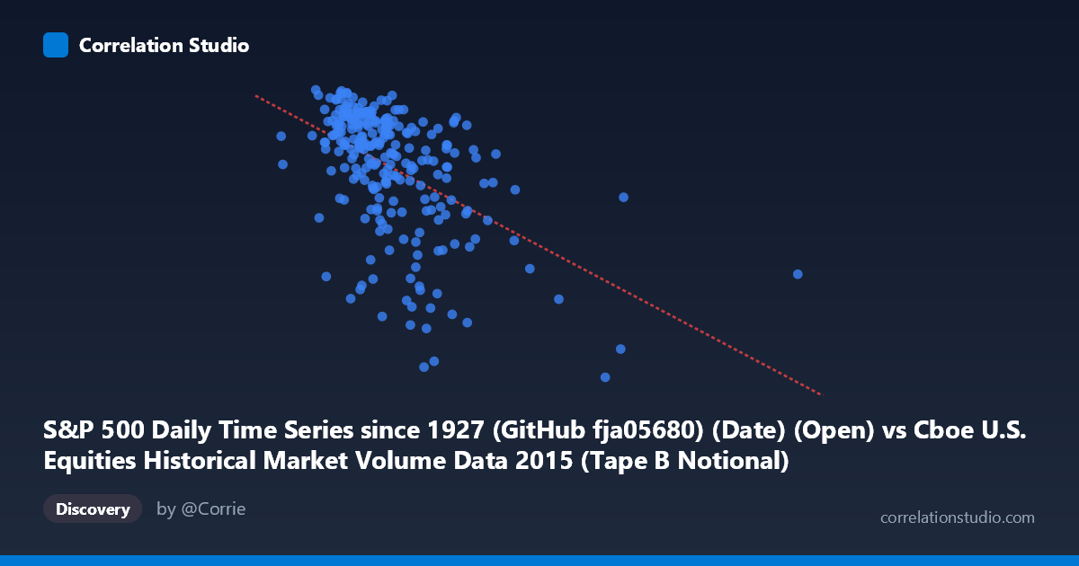
S&P 500 Daily Time Series since 1927 (GitHub fja05680) (Date) (Open) vs Cboe U.S. Equities Historical Market Volume Data 2015 (Tape B Notional)
- Pearson correlation (r)
- -0.4954
- Spearman correlation
- -0.5178
- p-value
- 0
- Sample size (n)
- 252
- 95% confidence interval
- -0.5833 to -0.396
- Granger causality
- X → Y
- Granger optimal lag
- 7
AI analysis
Analysis: S&P 500 Opening Price vs. Cboe Tape B Notional Volume (2015)
Relationship Overview The scatterplot reveals a moderate negative relationship between S&P 500 daily opening prices (X-axis, representing date/time as Unix-style timestamps spanning January–December 2015) and Cboe Tape B notional trading volume (Y-axis). As the year progresses, S&P 500 opening prices tend to decline while notional volume patterns shift accordingly. The linear regression equation y = -1.55×10⁻⁸x + 2146.03 captures a gentle downward slope, consistent with the S&P 500's well-documented mid-to-late 2015 correction, particularly the August selloff. The relationship is visually apparent but far from deterministic, with considerable vertical scatter throughout.
Correlation Strength and Statistical Significance The Pearson correlation of r = -0.4954 indicates a moderate negative association. However, the R² of 0.245 means that temporal progression (proxied by the date timestamp) explains only about 24.5% of the variance in Tape B notional volume — leaving roughly three-quarters of variability unexplained by this linear relationship alone. The 95% confidence interval of [-0.583, -0.396] is entirely negative and reasonably tight, confirming directional reliability, while the p-value of ~0 (against N = 3,302) confirms this is not a chance finding. Critically, Granger causality runs unidirectionally from X→Y (F = 2.19, p = 0.036) with an optimal lag of 7 trading days, suggesting that S&P 500 price levels have modest but statistically meaningful temporal predictive power over subsequent Tape B notional volume — though the Y→X direction is clearly non-significant (p = 0.478), ruling out reverse causation in this framework.
Notable Patterns, Clusters, and Outliers Several structural features stand out in the data. A dense cluster exists in the X range of approximately 3.2–5.5 billion (roughly Q1–Q2 2015) where Y values are relatively elevated and tightly packed between ~2050–2130, reflecting the S&P 500's relative stability and high Tape B activity in early 2015. A clear dispersion emerges at higher X values (mid-to-late 2015), where Y values drop sharply and spread widely, consistent with August's volatility spike and the subsequent choppy recovery. Several notable low-Y outliers appear — points around (6.8B, 1887), (6.1B, 1920), (5.96B, 1942), and (7.35B, 1929) — likely corresponding to specific high-volatility sessions during the August 2015 correction when index prices fell dramatically. One high-X outlier near 17.9 billion appears isolated at the far right, potentially a data artifact or an unusual late-December session worth verifying.
Confounding Factors and Caveats Several important caveats apply. First, the X-axis encodes dates as timestamps, so this correlation is partly measuring time-series trend rather than a direct causal price-volume mechanism — the negative relationship may largely reflect the calendar effect of the 2015 bear market occurring later in the year. Second, Tape B notional value is sensitive to both price levels and share volume simultaneously; since notional = price × shares, a falling S&P 500 mechanically reduces notional values even if share volume is unchanged, introducing mathematical coupling between the variables. Third, macroeconomic events (Fed rate hike expectations, China slowdown fears, oil price decline) drove both S&P price declines and volatility spikes simultaneously in H2 2015, acting as common confounders. Finally, while Granger causality is statistically present, its economic magnitude (F = 2.19) is modest, and Granger causality does not imply true structural causation.
Actionable Insights and Further Investigation Despite these caveats, the Granger result with a 7-period lag is practically interesting: it suggests that S&P 500 price levels may provide a roughly one-to-two week leading signal for Tape B notional activity, which could inform short-term liquidity and market-making strategies on Cboe. To sharpen this analysis, investigators should: (1) decompose the correlation by separating the time-trend component (e.g., detrending both series) to isolate a genuine price-volume relationship from pure calendar effects; (2) segment the dataset into pre- and post-August correction regimes to test whether the relationship is structurally stable; (3) control for the VIX or realized volatility, which almost certainly mediates the volume surge during the selloff; and (4) extend the Granger analysis to other Tape designations (A, C) to determine whether the predictive relationship is specific to Tape B or systemic across the broader market.
X dataset: Cboe U.S. Equities Historical Market Volume Data 2015
Y dataset: S&P 500 Daily Time Series since 1927 (GitHub fja05680) (Date)
Part of experiment: Daily - Cboe U.S. Equities Historical Market Volume Data 2015 vs S&P 500 Daily Time Series since 1927 (GitHub fja05680) (Date)