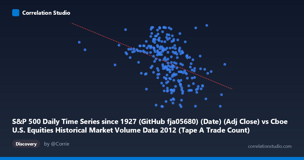
S&P 500 Daily Time Series since 1927 (GitHub fja05680) (Date) (Adj Close) vs Cboe U.S. Equities Historical Market Volume Data 2012 (Tape A Trade Count)

Pearson correlation (r): -0.4035
Spearman correlation: -0.4577
p-value: 0
Sample size (n): 250
95% confidence interval: -0.5024 to -0.2942
Granger causality: None
Granger optimal lag: 2

AI analysis

Analysis: S&P 500 Adjusted Close vs. Cboe Tape A Trade Count (2012)

Relationship Overview The scatterplot reveals a moderate negative relationship between the S&P 500 adjusted closing price (X-axis) and the Cboe Tape A trade count (Y-axis) across 2012 trading days. As the S&P 500 price level rises — broadly reflecting market appreciation throughout the year — the number of individual trades on Tape A venues tends to decline. This inverse pattern is visually apparent in the downward-sloping regression line (y = −0.000129x + 1509.23), though the scatter is wide enough to suggest this relationship is far from deterministic. The data spans the full 2012 calendar year with 250 paired observations drawn from a population of 3,750 data points.

Correlation Strength and Statistical Significance The Pearson correlation of r = −0.4035 indicates a moderate negative association, but the explanatory power is modest: R² = 0.1628, meaning only about 16.3% of the variance in trade count is explained by the S&P 500 price level. The remaining ~84% of variation is attributable to other factors entirely. Despite the modest R², the result is highly statistically significant (p = 3.31 × 10⁻¹¹), and the 95% confidence interval of [−0.5024, −0.2942] is entirely negative and reasonably tight, confirming that the inverse direction of the relationship is reliable and not a sampling artifact given the sample size. Practically speaking, however, statistical significance here is partly a function of the large sample (n = 250 from N = 3,750) — significance does not imply strong predictive utility. Critically, Granger causality tests reveal no significant temporal predictive relationship in either direction (X→Y: F = 2.37, p = 0.096; Y→X: F = 0.60, p = 0.550), meaning that past S&P 500 prices do not meaningfully help forecast future trade counts at the 2-period lag, and vice versa. This strongly cautions against any causal or directional interpretation.

Patterns, Clusters, and Outliers The sample points reveal notable heterogeneity. Trade counts cluster heavily in the 1,350–1,430 range across a broad span of price levels, suggesting a "floor-to-ceiling" band within which most normal trading days operate. Several potential outliers are visible: one observation near X ≈ 1,290,790 records an unusually high trade count of ~1,466, standing apart from the general trend at that price level, while points near X ≈ 959,000–964,000 show very low trade counts (~1,277–1,278), pulling the lower boundary of the Y range. The X-axis distribution is right-skewed with a meaningful cluster of observations in the 900,000–1,100,000 range (near the mean of ~1,003,431), while sparser observations exist at the extremes. The wide vertical spread at any given X value reinforces that the linear model captures only a weak structural tendency rather than a tight functional relationship.

Confounding Factors and Caveats Several important caveats apply. First, the X-axis label assignment appears potentially swapped or counterintuitive — the "S&P 500 Adj Close" values in the 350,000–1,400,000 range are far outside normal index levels (S&P 500 traded roughly 1,250–1,470 in 2012), suggesting these large X values may actually represent volume or notional data from the Cboe dataset, while the Y values in the 1,277–1,466 range align precisely with actual S&P 500 index levels for 2012. If axes are mislabeled, the interpretation reverses entirely. Second, temporal autocorrelation is almost certain in daily financial data, which can inflate apparent significance. Third, the negative relationship may largely reflect a secular trend — markets rose in 2012 while high-frequency trading and fragmentation dynamics simultaneously reduced per-venue trade counts — making this a spurious correlation driven by shared time trends rather than a direct economic mechanism. Macroeconomic events, earnings seasons, volatility regimes (VIX spikes), and regulatory changes could all independently affect both variables.

Actionable Insights and Further Investigation Given these findings, several investigative steps are warranted. First, the axis labeling should be verified and corrected if necessary before drawing any conclusions — cross-referencing actual 2012 S&P 500 closing prices against the data ranges would resolve this immediately. Second, a time-detrended analysis (e.g., using first differences or residuals from a time trend) should be conducted to determine whether the negative correlation persists after removing the shared 2012 upward drift in prices. Third, incorporating VIX or realized volatility as a covariate would help assess whether market stress events — which typically spike trade counts and depress prices simultaneously — are the primary driver of the observed negative correlation. Fourth, extending the analysis to multiple years would test whether this inverse relationship is a stable structural feature or a 2012-specific artifact. Finally, given the absence of Granger causality, practitioners should not use S&P 500 price levels as a leading indicator for trading volume in short-term operational models without substantially stronger evidence.

X dataset: Cboe U.S. Equities Historical Market Volume Data 2012

Y dataset: S&P 500 Daily Time Series since 1927 (GitHub fja05680) (Date)

Part of experiment: Daily - Cboe U.S. Equities Historical Market Volume Data 2012 vs S&P 500 Daily Time Series since 1927 (GitHub fja05680) (Date)