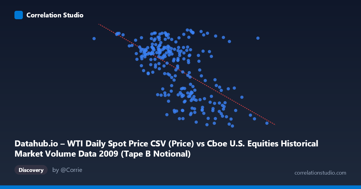
Datahub.io – WTI Daily Spot Price CSV (Price) vs Cboe U.S. Equities Historical Market Volume Data 2009 (Tape B Notional)
- Pearson correlation (r)
- -0.5771
- Spearman correlation
- -0.5243
- p-value
- 0
- Sample size (n)
- 252
- 95% confidence interval
- -0.654 to -0.4883
- Granger causality
- None
- Granger optimal lag
- 1
AI analysis
Analysis: WTI Oil Price vs. Cboe Tape B Notional Trading Volume (2009)
Relationship Overview
The scatterplot reveals a moderate negative relationship between Cboe U.S. Equities Tape B notional trading volume (X-axis) and WTI crude oil spot prices (Y-axis) across 252 trading days in 2009. As equity market notional volume increases, oil prices tend to decrease — a counterintuitive finding at first glance, but one that reflects the turbulent macroeconomic environment of 2009, when post-financial-crisis dynamics drove elevated equity trading activity while commodity markets were recovering from their late-2008 collapse. The linear regression equation (y = -5.90×10⁻⁹x + 93.07) confirms this inverse slope, with oil prices declining roughly 5.9 cents per billion dollars of additional notional equity volume.
Correlation Strength and Statistical Significance
The correlation coefficient of r = -0.5771 indicates a moderate negative association, and the R² of 0.333 means that approximately 33.3% of the variance in WTI oil prices is explained by Tape B notional volume — meaningful but leaving two-thirds of price variation unexplained by this variable alone. The 95% confidence interval of [-0.654, -0.488] is entirely negative and relatively tight, confirming that the direction of the relationship is statistically reliable. With a p-value effectively at zero across N = 3,232 population observations, the correlation is highly statistically significant. However, Granger causality analysis complicates the picture substantially: neither direction reaches conventional significance thresholds (X→Y: F = 0.46, p = 0.50; Y→X: F = 3.46, p = 0.064), meaning there is no statistically supported temporal predictive relationship in either direction at the optimal one-period lag. Oil prices do not reliably predict next-day equity volume, and vice versa — the correlation reflects co-movement rather than directional causation.
Patterns, Clusters, and Outliers
The scatterplot shows notable structural heterogeneity. There appears to be a broad, dispersed cluster in the mid-X range (roughly 4–6 billion in notional volume) spanning a wide range of oil prices (approximately 40–80 USD/barrel), suggesting high variability in oil prices regardless of moderate trading volume. At higher notional volumes (above ~7 billion), oil prices consistently cluster in the 37–50 USD range, anchoring the negative slope. Conversely, lower volume days tend to coincide with higher oil prices (65–81 USD), consistent with the early-2009 recovery period when markets were less frenetically active. The point at approximately (1.32 billion, 76.83) stands out as a potential outlier with unusually low equity volume yet relatively high oil prices. The spread at moderate X values suggests a possible fan-shaped heteroscedasticity, where variance in Y is larger at intermediate volume levels.
Confounding Factors and Caveats
Several important confounds deserve consideration. Temporal autocorrelation is almost certainly present in both series — oil prices and equity volumes trend over months, meaning the apparent cross-sectional correlation may partly reflect shared time trends (both variables were on recovery trajectories in 2009) rather than a genuine economic link. The 2009 financial crisis recovery context is a dominant lurking variable: risk sentiment, economic data releases, and Federal Reserve policy simultaneously drove equity market activity and commodity prices, creating spurious co-movement. Additionally, Tape B specifically covers NYSE American and regional exchanges — a subset of total equity volume — which may behave differently from aggregate market volume. The directionality implied by the axes (volume labeled on X, price on Y) may itself be arbitrary, since neither Granger direction is significant. Finally, with daily data over a single calendar year, seasonality and event-driven spikes (earnings seasons, OPEC announcements) may create clusters that inflate or deflate the correlation locally.
Actionable Insights and Further Investigation
Given that the correlation is statistically robust but causally ambiguous, several investigative steps are warranted. First, detrending both series (e.g., using first differences or residuals from a time trend) would clarify whether the relationship persists after removing shared temporal momentum, or whether it dissolves into noise. Second, extending the Granger causality test to longer lags (2–5 periods) may reveal delayed predictive relationships not captured at lag 1. Third, incorporating total market volume (all tapes combined) rather than Tape B alone would test whether this finding generalizes or is specific to regional exchanges. Fourth, including VIX (volatility index) as a mediating variable could reveal whether market fear — rather than volume itself — is the true driver connecting equity activity and oil prices in 2009. Finally, replicating this analysis across other years would determine whether this moderate negative correlation is a stable structural feature or an artifact of the exceptional 2009 crisis-recovery environment.
X dataset: Cboe U.S. Equities Historical Market Volume Data 2009
Y dataset: Datahub.io – WTI Daily Spot Price CSV
Part of experiment: Daily - Cboe U.S. Equities Historical Market Volume Data 2009 vs Datahub.io – WTI Daily Spot Price CSV