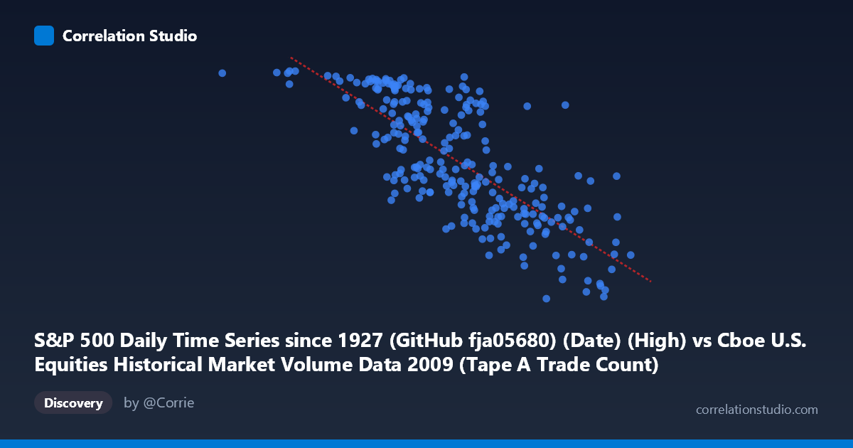
S&P 500 Daily Time Series since 1927 (GitHub fja05680) (Date) (High) vs Cboe U.S. Equities Historical Market Volume Data 2009 (Tape A Trade Count)
- Pearson correlation (r)
- -0.7655
- Spearman correlation
- -0.7748
- p-value
- 0
- Sample size (n)
- 252
- 95% confidence interval
- -0.8122 to -0.709
- Granger causality
- X → Y
- Granger optimal lag
- 10
AI analysis
Analysis: S&P 500 Daily High vs. Cboe Tape A Trade Count (2009)
Relationship Overview The scatterplot reveals a moderately strong negative relationship between the S&P 500 daily high price (X) and the Cboe Tape A trade count (Y) across 2009 trading days. As the S&P 500's daily high increases, the number of individual trades on Tape A (NYSE-listed securities) tends to decrease. This inverse pattern reflects a well-documented market dynamic: during the crisis-driven, high-volatility early months of 2009, when index prices were depressed (X values clustered in the 700–1,300 range), trading activity was frenetic. As prices recovered through the year, markets calmed and trade counts declined. The linear regression equation y = −0.00022207x + 1318.17 captures this downward slope, though the relationship is clearly not purely linear across the full range.
Correlation Strength and Statistical Robustness The Pearson correlation of r = −0.7655 indicates a strong negative association, and the R² of 0.5860 means that approximately 58.6% of the variance in Tape A trade counts is explained by the S&P 500 daily high level alone — a substantial but incomplete explanation, leaving ~41% attributable to other factors. The 95% confidence interval of [−0.8122, −0.7090] is reassuringly tight and entirely negative, confirming the direction is not a statistical artifact. With a p-value reported as 0 (effectively p < 0.0001) and n = 252 paired observations drawn from a population of N = 3,232, the result is highly significant. Critically, the Granger causality test supports a unidirectional temporal relationship: X Granger-causes Y (F = 1.94, p = 0.041) at an optimal lag of 10 trading periods (~2 weeks), while Y does not Granger-cause X (F = 1.50, p = 0.141). This suggests that movements in S&P 500 price levels carry predictive information about future trade counts, but trade count activity does not similarly predict future price levels — a meaningful asymmetry for practitioners.
Notable Patterns, Clusters, and Outliers Several structural features stand out in the data. There is a visible cluster of high trade counts (Y ≈ 1,050–1,130) concentrated at lower X values (~700–1,300), corresponding to the market trough period of early 2009 when fear and forced selling drove exceptional fragmentation of order flow. A second looser cluster sits at mid-to-high X values (~1,600–2,000) with moderate trade counts (~850–1,000), reflecting the recovery phase. The point near X ≈ 362,081 with Y ≈ 1,126 appears as an extreme outlier on the left tail — potentially a data artifact, a mis-scaled entry, or a special trading session — and warrants verification. Similarly, the highest X values (~2,400–2,550) show the lowest trade counts (~700–780), consistent with the trend but forming a sparse right-tail cluster. The scatter also shows heteroscedasticity: variance in Y is noticeably wider at lower X values, suggesting the relationship is noisier during stressed market conditions.
Confounding Factors and Interpretive Caveats This correlation is heavily confounded by time: both variables are jointly driven by the extraordinary market conditions of 2009, spanning the post-Lehman crisis trough (March 2009 low ~666 on S&P) and subsequent recovery. The negative correlation may largely be a proxy for the passage of time — prices rose and volatility fell as the year progressed, while high-frequency and retail participation normalized. Tape A trade count is also influenced by factors entirely independent of price level, including exchange fee structures, market microstructure changes, the proliferation of algorithmic trading, and regulatory events specific to 2009 (e.g., SEC dark pool scrutiny). The Granger causality result, while statistically significant, uses a modest F-statistic (1.94) and should not be over-interpreted as economic causation — it reflects temporal precedence, not mechanism. Additionally, using daily high as the price variable rather than close or VWAP introduces intraday noise.
Actionable Insights and Further Investigation Practitioners could explore whether the 10-period Granger lag has tactical utility — if rising index highs predict declining trade fragmentation two weeks forward, this could inform execution strategy (e.g., anticipating reduced liquidity fragmentation during trending markets). For deeper insight, analysts should partial out the time trend by including a date variable in a multivariate regression to isolate whether the price–trade-count relationship holds within market regimes, not just across them. It would also be valuable to replicate this analysis across other years (e.g., 2007–2008, 2010–2011) to determine whether the relationship is specific to 2009's unique conditions or a structural feature of U.S. equity market microstructure. Finally, the outlier near X = 362,081 should be investigated and potentially excluded before drawing further conclusions, as it may be distorting both the regression slope and correlation magnitude.
X dataset: Cboe U.S. Equities Historical Market Volume Data 2009
Y dataset: S&P 500 Daily Time Series since 1927 (GitHub fja05680) (Date)
Part of experiment: Daily - Cboe U.S. Equities Historical Market Volume Data 2009 vs S&P 500 Daily Time Series since 1927 (GitHub fja05680) (Date)