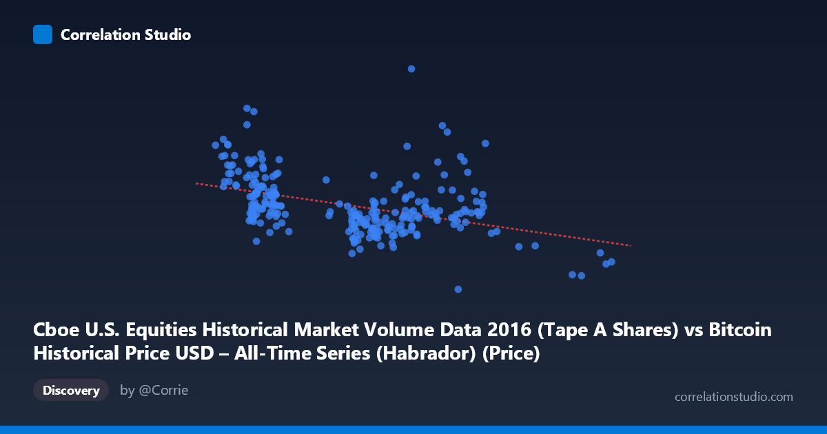
Cboe U.S. Equities Historical Market Volume Data 2016 (Tape A Shares) vs Bitcoin Historical Price USD – All-Time Series (Habrador) (Price)
- Pearson correlation (r)
- -0.4251
- Spearman correlation
- -0.4161
- p-value
- 0
- Sample size (n)
- 252
- 95% confidence interval
- -0.5213 to -0.3182
- Granger causality
- None
- Granger optimal lag
- 10
- Time coverage
- 2016-01-04 to 2016-12-30
- Recomputed on refreshed data
- 2026-10-24 (r was -0.4251)
AI analysis
Analysis: Cboe Equities Volume vs. Bitcoin Price (2016)
1. Relationship Overview
The scatterplot displays a moderate negative association between Cboe U.S. equities market volume (X-axis) and Bitcoin's price (Y-axis) throughout 2016. As equity trading volume increases, Bitcoin price tends to decrease, though the relationship shows substantial scatter rather than a tight linear pattern. The data points cluster primarily in the X range of 400–750, with a mean volume of 567 and a Bitcoin price mean of roughly $272 million (likely a data-scaling artifact, as this exceeds actual 2016 BTC prices by orders of magnitude — see caveats below).
2. Strength, Direction, and Statistical Confidence
The correlation coefficient (r = -0.4251) indicates a moderate negative relationship, but the r² of 0.1807 reveals that only 18% of the variance in Bitcoin price is explained by equity volume — leaving over 80% attributable to other factors. The 95% CI [-0.5213, -0.3182] is reasonably tight and entirely negative, and the p-value (1.77E-12) confirms this correlation is highly statistically significant and not due to chance. However, statistical significance does not imply strong predictive power — the modest r² means this relationship, while real, is not strong enough for reliable point forecasting.
Critically, the Granger causality tests show no significant predictive direction in either direction (X→Y: p=0.54; Y→X: p=0.96). This means neither variable's past values help forecast the other's future values in a time-series sense. The static correlation may reflect a contemporaneous association (both responding to a shared macro driver) rather than one variable causally leading the other — an important distinction for any trading or forecasting application.
3. Notable Patterns and Outliers
The scatter shows a loose downward-sloping cloud rather than a clean linear trend. Lower X-values (358–450) tend to associate with higher Y-values (270M–360M range), while mid-to-high X-values (600–750) cluster in a lower Y-band (200M–260M). A few outliers stand out: the point at (833.10, 190M) — the highest X-value in the sample — sits notably low on Y, potentially exerting leverage on the regression line. Similarly, (531.80, 322M) deviates upward from the general trend at that X-range. These outliers, combined with the wide vertical spread at any given X-value (e.g., X≈420 spans Y from 244M to 363M), suggest a weak, noisy linear fit rather than a robust deterministic relationship.
4. Confounding Factors and Caveats
Several caveats warrant attention:
- Data scaling inconsistency: The Y-axis values (hundreds of millions) are inconsistent with known 2016 Bitcoin prices (~$400–$970), suggesting a metadata/column mismatch or unit scaling error in the dataset — this should be verified before drawing economic conclusions. - Spurious correlation risk: Both series are time-ordered financial data from the same calendar year; shared exposure to broader market sentiment, seasonality, or macroeconomic events (rather than a direct causal link between equity volume and BTC price) could drive the observed correlation. - Non-stationarity: Financial time series often trend over time; if both variables have underlying trends (e.g., BTC's 2016 bull run, equity volume seasonality), this can inflate correlation without genuine relationship. - Sample vs. population: n=252 paired points drawn from a population of 3,622 — sampling methodology (e.g., matching by date) should be checked for consistency.
5. Recommendations
1. Verify data integrity — confirm the Y-axis column truly represents Bitcoin price and check for unit/scaling errors given the implausible magnitude. 2. Detrend or difference both series before correlating to rule out spurious trend-driven correlation, then re-test r² and Granger causality on stationary series. 3. Investigate lagged/nonlinear relationships beyond linear Pearson correlation and the tested lag structure (e.g., variable lag windows, cross-correlation function) since Granger tests were insignificant only at lag 10. 3. Explore shared confounders (e.g., VIX, USD index, macro news events) that could jointly explain movements in both equity volume and BTC price. 4. Given the low r² and lack of Granger causality, avoid using this relationship for predictive trading models — treat it as a weak associative signal at best, suitable for exploratory context rather than forecasting.
X dataset: Bitcoin Historical Price USD – All-Time Series (Habrador)
Y dataset: Cboe U.S. Equities Historical Market Volume Data 2016
Part of experiment: Bitcoin - Bitcoin Historical Price USD – All-Time Series (Habrador) vs Cboe U.S. Equities Historical Market Volume Data 2016