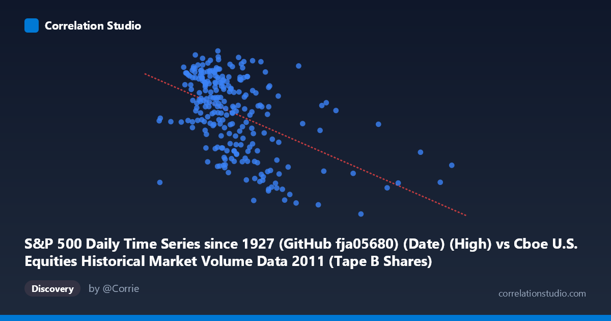
S&P 500 Daily Time Series since 1927 (GitHub fja05680) (Date) (High) vs Cboe U.S. Equities Historical Market Volume Data 2011 (Tape B Shares)
- Pearson correlation (r)
- -0.4902
- Spearman correlation
- -0.4815
- p-value
- 0
- Sample size (n)
- 252
- 95% confidence interval
- -0.5787 to -0.3902
- Granger causality
- None
- Granger optimal lag
- 1
AI analysis
Analysis: S&P 500 High vs. Cboe Tape B Share Volume (2011)
Relationship Overview The scatterplot reveals a moderate negative relationship between the S&P 500 daily high price and Cboe Tape B share volume throughout 2011. As the S&P 500 high increases, Tape B share volume tends to decline, following the linear regression equation y = -8.67×10⁻⁷x + 1362.31. This pattern is consistent with a well-documented market phenomenon: during periods of elevated equity prices, trading volume in certain market segments tends to contract, while market stress and price declines are often accompanied by heightened trading activity. The relationship is visually apparent as a downward-sloping cloud of points, though with considerable scatter around the regression line.
Correlation Strength and Statistical Significance The Pearson correlation of r = -0.4902 indicates a moderate negative association, but the explanatory power deserves careful framing: r² = 0.2403 means only 24% of the variance in Tape B share volume is explained by the S&P 500 high, leaving 76% attributable to other factors. The 95% confidence interval of [-0.5787, -0.3902] is entirely negative and does not cross zero, lending strong directional confidence. The p-value of 2.22×10⁻¹⁶ confirms the relationship is highly statistically significant and extremely unlikely to be a chance artifact given n = 252 paired observations from a population of N = 3,780. However, statistical significance should not be conflated with practical magnitude — the moderate r² tempers enthusiasm for predictive applications. Critically, Granger causality tests find no significant predictive directionality in either direction (X→Y: F = 0.082, p = 0.776; Y→X: F = 0.008, p = 0.931), meaning that neither variable meaningfully predicts the other's future values at a one-period lag. The relationship appears contemporaneous rather than leading/lagging, which substantially limits its utility for forecasting.
Notable Patterns, Clusters, and Outliers Several structural features are visible in the data. There is a dense cluster of points in the mid-range of X (roughly 65M–130M in S&P high values) with Tape B volume spanning approximately 1,150–1,370, reflecting the bulk of 2011 trading days. A notable right-tail dispersion is evident, with several points extending toward X values of 165M–265M (corresponding to later 2011 dates when the S&P recovered from the summer correction) that appear to anchor the negative slope. Points such as approximately (189M, 1186) and (176M, 1281) behave as moderate high-leverage observations. The vertical spread at any given X value is substantial — on the order of 150–200 units — indicating considerable heteroscedasticity and reinforcing that X alone is a weak predictor. There is no obvious non-linear curvature, suggesting a linear model is a reasonable first approximation, though the wide residual band warrants caution.
Confounding Factors and Interpretive Caveats Several important caveats apply. First, 2011 was an atypical market year, characterized by the August debt-ceiling crisis, S&P's U.S. credit downgrade, and European sovereign debt fears — episodic volatility spikes may be driving the correlation as much as any structural relationship. Second, Tape B specifically covers NYSE American (AMEX) and regional exchange listings, meaning it reflects a subset of market activity that may respond differently to index-level price changes than total market volume. Third, the X-axis variable is labeled as S&P 500 high (not close or open), introducing intraday range dynamics that may add noise. Fourth, both variables are time-indexed over the same year, raising the possibility that shared temporal trends (e.g., a declining market in H1 with high volume followed by recovery in H2 with lower volume) are generating the correlation rather than a fundamental economic mechanism — this is essentially a spurious co-movement driven by the market's 2011 trajectory. The absence of Granger causality supports this interpretation.
Actionable Insights and Further Investigation Given the moderate but not explanatory correlation and absent temporal causality, several follow-up analyses are warranted. Decomposing the time series into trend and cyclical components would help isolate whether the correlation persists after removing the 2011 market arc or disappears as a trend artifact. Extending the analysis across multiple years (the S&P dataset dates to 1927) would test whether r ≈ -0.49 is stable or regime-dependent. Incorporating VIX or realized volatility as a covariate could reveal whether the negative price-volume relationship is mediated by volatility — a known driver of retail and institutional trading behavior. Analysts should also examine whether other Tape segments (A, C) show similar patterns, which would clarify whether this is a market-wide phenomenon or Tape B-specific. Finally, given the 76% unexplained variance, building a multivariate model incorporating day-of-week effects, macroeconomic announcements, and cross-exchange volume flows would yield substantially more explanatory and potentially actionable insight.
X dataset: Cboe U.S. Equities Historical Market Volume Data 2011
Y dataset: S&P 500 Daily Time Series since 1927 (GitHub fja05680) (Date)
Part of experiment: Daily - Cboe U.S. Equities Historical Market Volume Data 2011 vs S&P 500 Daily Time Series since 1927 (GitHub fja05680) (Date)