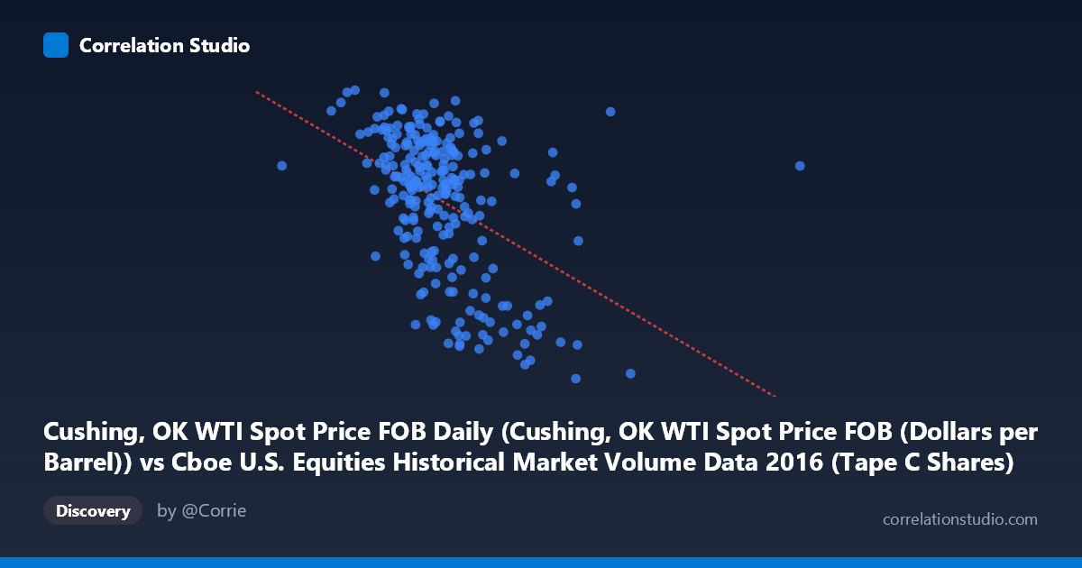
Cushing, OK WTI Spot Price FOB Daily (Cushing, OK WTI Spot Price FOB (Dollars per Barrel)) vs Cboe U.S. Equities Historical Market Volume Data 2016 (Tape C Shares)
- Pearson correlation (r)
- -0.449
- Spearman correlation
- -0.4589
- p-value
- 0
- Sample size (n)
- 252
- 95% confidence interval
- -0.5425 to -0.3446
- Granger causality
- None
- Granger optimal lag
- 1
AI analysis
Analysis: WTI Crude Oil Prices vs. Cboe Tape C Share Volume (2016)
Relationship Overview
The scatterplot reveals a negative relationship between WTI crude oil spot prices (X-axis) and Cboe Tape C equity share volumes (Y-axis) across 252 trading days in 2016. As oil prices rise, Tape C share volumes tend to decline, and vice versa. The linear regression equation (y = -1.11125E⁻⁰⁷x + 58.07) confirms this inverse slope, suggesting that for every ~$9/barrel increase in WTI prices, Tape C volumes decline by roughly one unit. Visually, the cloud of points tilts downward from left to right, though with considerable scatter throughout, indicating the relationship is real but far from deterministic.
Correlation Strength and Statistical Significance
The correlation coefficient of r = -0.449 indicates a moderate negative association. However, R² = 0.202 means that only about 20% of the variance in Tape C share volumes is statistically explained by WTI prices — leaving roughly 80% attributable to other factors. The 95% confidence interval of [-0.543, -0.345] is meaningfully narrow and sits entirely in negative territory, providing strong confidence that the true population correlation is genuinely negative rather than an artifact of sampling. The p-value of 6.6E-14 is extraordinarily small, making it statistically beyond doubt that this correlation is non-zero given the sample of 252 and population of 3,622. That said, Granger causality tests show no significant temporal predictive direction in either direction (X→Y: F=1.57, p=0.211; Y→X: F=0.21, p=0.644), meaning neither variable reliably predicts the other's future values at a one-period lag. This is a critical caveat: the correlation is real contemporaneously, but neither series can be said to lead the other.
Notable Patterns, Clusters, and Outliers
Several structural features stand out in the data. There appears to be a cluster of moderate-to-high volume observations (Y ≈ 44–51) concentrated in the lower oil price range (X ≈ $95M–$130M range in scaled units), consistent with early-to-mid 2016 when oil prices were depressed and equity market uncertainty was elevated. A distinct lower-right cluster is visible where oil prices are higher but volumes drop sharply (e.g., points near X=175M, Y≈29.6 and X=166M, Y≈33.2), suggesting specific periods — likely late 2016 oil price recoveries — where equity trading activity was notably subdued. A few potential outliers exist at high Y values with moderate X (e.g., Y≈51.4 at X≈99.8M), which may reflect specific volatility events driving anomalous volume spikes independent of oil prices.
Confounding Factors and Caveats
Interpreting this correlation requires significant caution. 2016 was an unusual year macroeconomically: it encompassed the tail end of an oil price crash, Brexit uncertainty, the U.S. presidential election, and Federal Reserve policy shifts — all of which independently influenced both oil markets and equity trading volumes. Tape C volume specifically reflects Nasdaq-listed securities, meaning sector composition (heavily technology) may have its own dynamics largely unrelated to oil. Furthermore, both variables are likely driven by common third factors — broad macroeconomic risk sentiment, volatility indices (VIX), or institutional trading patterns — creating spurious correlation. The absence of Granger causality also warns against any mechanistic interpretation. Finally, the daily granularity means autocorrelation within each series could inflate the apparent statistical significance, and the effective degrees of freedom may be lower than the raw n=252 implies.
Actionable Insights and Further Investigation
Despite the moderate correlation and lack of causal directionality, several follow-up analyses are warranted. Controlling for the VIX or broader market volatility measures would help isolate whether oil-volume co-movement persists after accounting for shared risk-appetite dynamics. A rolling correlation analysis over sub-periods of 2016 (pre/post-OPEC announcements, pre/post-election) could reveal whether the relationship is stable or episodic. Researchers should also test non-linear specifications (e.g., a regime-switching or polynomial model), as the scatter suggests the relationship may strengthen only at oil price extremes. Finally, expanding the analysis to multiple years would test whether this inverse relationship is a durable structural feature of 2016 specifically or a broader persistent phenomenon, which would significantly strengthen any practical trading or risk-management conclusions drawn from this data.
X dataset: Cboe U.S. Equities Historical Market Volume Data 2016
Y dataset: Cushing, OK WTI Spot Price FOB Daily
Part of experiment: Daily - Cboe U.S. Equities Historical Market Volume Data 2016 vs Cushing, OK WTI Spot Price FOB Daily