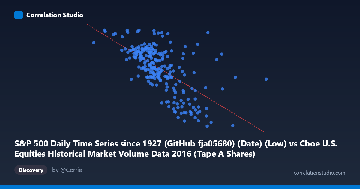
S&P 500 Daily Time Series since 1927 (GitHub fja05680) (Date) (Low) vs Cboe U.S. Equities Historical Market Volume Data 2016 (Tape A Shares)
- Pearson correlation (r)
- -0.6338
- Spearman correlation
- -0.6324
- p-value
- 0
- Sample size (n)
- 252
- 95% confidence interval
- -0.7024 to -0.5536
- Granger causality
- None
- Granger optimal lag
- 4
AI analysis
Analysis: S&P 500 Low Price vs. Cboe Tape A Share Volume (2016)
Relationship Overview The scatterplot reveals a moderate negative relationship between the S&P 500 daily low price (X-axis) and Cboe Tape A share volume (Y-axis) across 252 trading days in 2016. As the S&P 500 low price increases throughout the year, Tape A share volume tends to decline. This inverse pattern is visually apparent as a downward-sloping cloud of points, consistent with a well-documented market dynamic: rising equity prices are often accompanied by declining trading volume, while lower price levels — typically associated with volatility or uncertainty — tend to attract heavier trading activity.
Correlation Strength and Statistical Significance The Pearson correlation of r = -0.6338 indicates a moderate-to-strong negative association, and the R² of 0.4017 means that approximately 40.2% of the variance in Tape A share volume is explained by the S&P 500 low price level. While meaningful, this also implies that nearly 60% of the volume variation is driven by other factors. The 95% confidence interval of [-0.7024, -0.5536] is entirely negative and reasonably tight, reinforcing confidence that the inverse relationship is genuine and not an artifact of sampling. The p-value of effectively zero confirms high statistical significance across the population of N = 3,622. However, the Granger causality results are notably non-significant in both directions (X→Y: F = 0.61, p = 0.65; Y→X: F = 1.19, p = 0.32), meaning neither variable reliably predicts the other temporally at a 4-period lag. This is a critical caveat: the correlation reflects a co-movement or shared structural trend across 2016, not a predictive or causal mechanism in either direction.
Notable Patterns and Outliers Several features stand out in the data. The bulk of observations cluster between roughly 220–310M on the X-axis and 2,040–2,180 on the Y-axis, forming a relatively dense core. There are visible outliers at the extremes: points with very low S&P 500 lows (near 105–180M range, corresponding to early 2016's market turbulence) show elevated volume, while a few high-price, low-volume points populate the upper-right boundary. One striking outlier near (190M, 2,265) represents an unusually high volume day at a relatively modest price level — potentially a major news-driven or rebalancing event. The spread of points also appears to widen at lower X values, suggesting heteroscedasticity, where volume becomes more variable during lower-priced, more volatile market regimes.
Confounding Factors and Caveats Several confounds complicate a straightforward interpretation. Most importantly, both variables are likely driven by a common underlying factor: time. The S&P 500 broadly trended upward in 2016 after a volatile start, meaning the negative correlation may largely reflect a secular temporal trend — rising prices over the year coinciding with normalizing (declining) post-volatility volume — rather than a structural price-volume relationship. Additionally, market structure changes, such as shifts in algorithmic trading activity, quarterly expiration cycles, election-related volatility (November 2016), and Federal Reserve announcements, could independently drive both series. The Granger non-causality result strongly supports this interpretation: the apparent correlation is likely a spurious artifact of shared temporal drift rather than any direct functional link.
Actionable Insights and Further Investigation Given these findings, analysts should detrend both series before re-evaluating the correlation to isolate any genuine price-volume relationship from the shared time trend. It would be valuable to segment the data by market regime — separating the high-volatility Q1 period from the more stable Q2–Q4 — to test whether the negative correlation holds consistently across conditions or is regime-dependent. Incorporating additional volume metrics (e.g., Tape B and C shares, notional value, VIX as a control variable) would help isolate whether this relationship is specific to Tape A or reflects broader market-wide dynamics. Finally, extending the analysis across multiple years would clarify whether 2016's pattern is representative or idiosyncratic to that year's unusual macro environment, including the Brexit shock and U.S. presidential election.
X dataset: Cboe U.S. Equities Historical Market Volume Data 2016
Y dataset: S&P 500 Daily Time Series since 1927 (GitHub fja05680) (Date)
Part of experiment: Daily - Cboe U.S. Equities Historical Market Volume Data 2016 vs S&P 500 Daily Time Series since 1927 (GitHub fja05680) (Date)