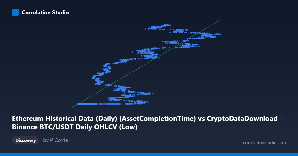
Ethereum Historical Data (Daily) (AssetCompletionTime) vs CryptoDataDownload – Binance BTC/USDT Daily OHLCV (Low)
- Pearson correlation (r)
- 0.8552
- Spearman correlation
- 0.89
- p-value
- 0
- Sample size (n)
- 3191
- 95% confidence interval
- 0.8456 to 0.8642
- Granger causality
- None
- Granger optimal lag
- 10
- Time coverage
- 2017-08-17 to 2026-05-20
AI analysis
Analysis of the Relationship Between X and Y Variables
1. Overview of the Visualization
The scatterplot depicts a strong positive association between the X variable (labeled as "Ethereum Historical Data" but containing what appears to be a completion-time or record-count metric ranging 2,817–123,084) and Y (labeled as Binance BTC/USDT daily "Low" price, ranging ~$1.61B–$1.78B — note these values are far outside realistic BTC price ranges, suggesting a units/scaling anomaly or mislabeled column). At low X values (roughly 3,000–20,000), Y clusters tightly near a floor of ~1,614,335,000–1,614,336,000, showing almost no variance. As X increases beyond ~20,000, Y rises steeply and with increasing dispersion, climbing toward 1,660M–1,780M. This produces a pattern that resembles a threshold/step function transitioning into a roughly linear or slightly convex rise, rather than a uniform straight-line relationship across the full range.
2. Strength, Direction, and Statistical Confidence
The Pearson correlation (r = 0.855) indicates a strong positive linear relationship, with r² = 0.731 meaning approximately 73% of the variance in Y is statistically explained by X — a substantial but not complete linear relationship, leaving ~27% of variance driven by other factors or nonlinearity. The 95% CI [0.846, 0.864] is narrow, reflecting high precision given the large sample (n = 3,191), and the p-value ≈ 0 confirms this correlation is not due to chance. However, correlation strength does not imply causation or predictive power over time: the Granger causality tests show no significant temporal predictive direction in either direction (X→Y: p = 0.357; Y→X: p = 0.190). This is a critical caveat — despite the strong contemporaneous statistical association, neither variable's past values help forecast the other's future values at the tested lag structure (10 periods), suggesting the relationship may be driven by a shared underlying trend (e.g., both increasing over the same calendar period) rather than a lead-lag causal mechanism.
3. Notable Patterns and Anomalies
The most striking feature is the flat "floor" cluster at low X values, where Y is essentially constant (~1,614,335,200–1,614,335,700) despite X varying from ~3,700 to ~23,000. This is not consistent with a simple linear model and likely reflects a data-generating artifact — e.g., a fixed timestamp or default value applied before a certain date/threshold, or the initial period of one dataset before real data collection began. Once X exceeds roughly 20,000–25,000, Y "breaks free" and begins tracking upward with much greater variance, including apparent local peaks (e.g., X≈65,712 → Y≈1,775M; X≈80,731 → Y≈1,778M) that don't monotonically increase — suggesting cyclical or seasonal components superimposed on the trend. This bimodal/regime-switching structure means a single linear regression (y = 1461.75x + 1.61e9) may be a reasonable global approximation but poorly represents the low-X regime, where residuals will be large in relative terms (though small in absolute terms given Y's scale).
4. Confounding Factors and Caveats
Several caveats warrant attention. First, the labeling is suspicious: Y is described as a BTC/USDT "Low" price, yet its values (~1.6–1.8 billion) are inconsistent with actual historical BTC prices (which have ranged roughly $3,000–$110,000). This strongly suggests Y is actually a Unix timestamp or another mismapped column, not a genuine price — meaning the "correlation" may simply reflect that both X and Y increase with calendar time (a classic spurious correlation from two time-indexed series). Second, since both variables likely trend with time, the observed r may largely capture a shared time trend rather than a substantive economic relationship — consistent with the null Granger causality result. Third, the flat floor segment indicates possible data quality issues (padding, defaults, or misaligned joins) that should be resolved before trusting the regression coefficients.
5. Recommendations for Further Investigation
Before drawing substantive conclusions, verify the actual column definitions and units for both X and Y — the Y-axis values look like Unix timestamps rather than prices, which would explain both the scale and the trend-driven correlation. If confirmed, this analysis should be re-run using proper price/volume metrics. Additionally, given the null Granger causality result, avoid using either series to forecast the other in a trading or predictive context. Instead, consider: (a) detrending both series (e.g., differencing or removing a time trend) and re-testing correlation and Granger causality on residuals to isolate any genuine relationship beyond shared drift; (b) segmenting the analysis by regime (the flat low-X cluster vs. the rising high-X segment) to fit piecewise models; and (c) investigating the specific dates corresponding to the flat-Y cluster to diagnose the data anomaly at its source.
X dataset: CryptoDataDownload – Binance BTC/USDT Daily OHLCV
Y dataset: Ethereum Historical Data (Daily)
Part of experiment: Bitcoin - CryptoDataDownload – Binance BTC/USDT Daily OHLCV vs Ethereum Historical Data (Daily)