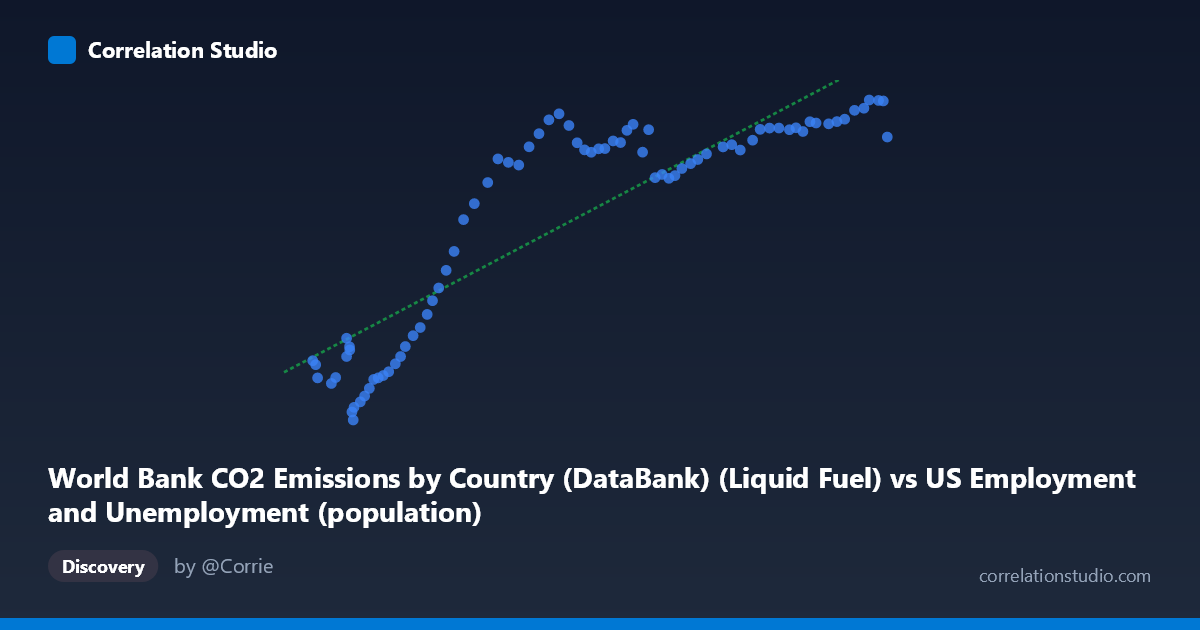
World Bank CO2 Emissions by Country (DataBank) (Liquid Fuel) vs US Employment and Unemployment (population)
- Pearson correlation (r)
- 0.8772
- Spearman correlation
- 0.8748
- p-value
- 0
- Sample size (n)
- 80
- 95% confidence interval
- 0.8145 to 0.9197
- Granger causality
- None
- Granger optimal lag
- 10
AI analysis
Scatterplot Analysis: US Liquid Fuel CO2 Emissions vs. US Population (1941–2020)
Relationship Overview
The scatterplot reveals a strong, positive relationship between US liquid fuel CO2 emissions (X-axis) and US population (Y-axis) across eight decades of annual data. As emissions increase from roughly 93,000 to 260,000 units, population rises correspondingly from approximately 2,500 to 13,600 units. The linear regression equation (y = 0.0629x − 1,184.24) captures this upward trend well across most of the observed range, though the scatter widens noticeably at higher emission values, suggesting the relationship becomes less uniform as both variables grow. The data broadly traces what appears to be a historical growth trajectory, with lower-emission, lower-population observations clustering at the left and higher values spreading rightward.
Correlation Strength and Statistical Interpretation
The Pearson correlation of r = 0.877 indicates a strong positive association, and the R² of 0.770 means that approximately 77% of the variance in US population is statistically explained by variation in liquid fuel CO2 emissions within this dataset. The 95% confidence interval for r [0.815, 0.920] is relatively tight and excludes zero entirely, and the p-value of effectively zero confirms this is not a chance result at any conventional significance threshold across n = 80 paired observations. However, the Granger causality analysis tells a critically important story: neither variable significantly predicts the other in a temporal lead-lag sense (X→Y: F = 1.03, p = 0.43; Y→X: F = 1.10, p = 0.38), even at an optimal lag of 10 periods. This means that while the two series move together strongly, neither emissions nor population demonstrably drives the other forward in time — the correlation is almost certainly driven by a shared underlying trend rather than any direct causal mechanism.
Notable Patterns, Clusters, and Outliers
The data exhibits two visually distinct regions: a lower-left cluster of points (roughly X < 130,000) where both variables are low and scatter is relatively tight, corresponding to earlier decades when both population and emissions were smaller; and a right-side spread (X 180,000) where Y values plateau somewhat between approximately 11,000 and 13,600, producing a subtle flattening or "ceiling" effect. This plateau suggests that population growth may have decelerated relative to emissions in more recent decades. A few notable outliers are visible — particularly points near (93,220; 4,555) and (260,329; 12,317), where the latter appears slightly below the regression line, consistent with the plateau behavior. The point at (104,995; 2,497) represents the lowest population observation and sits near the regression line, anchoring the lower end.
Confounding Factors and Interpretive Caveats
The most important caveat here is the spurious correlation problem: both US population and US liquid fuel CO2 emissions have trended upward over the 20th century primarily because of the passage of time and general economic and demographic growth. This is a textbook case of two non-stationary time series sharing a common temporal trend, which mechanically inflates correlation coefficients regardless of any true relationship. The dataset labels also warrant scrutiny — the X-axis is drawn from an "US Employment and Unemployment" dataset yet represents CO2 emissions, and the Y-axis is labeled as "population" but drawn from a CO2 emissions dataset, suggesting possible data joining or labeling ambiguity that should be verified before interpretation. Additionally, global events such as WWII-era rationing, the 1970s oil crises, the 2008 recession, and COVID-19 likely created short-term deviations invisible in aggregated annual trends. The Granger test's insignificance at lag 10 also raises the possibility that both series are independently driven by GDP, industrialization, or energy policy rather than each other.
Actionable Insights and Further Investigation
Given the strong correlation but absent Granger causality, the most productive next steps would be to detrend both series (e.g., first-differencing or HP filtering) and re-examine the correlation to determine how much persists beyond the shared time trend. Researchers should also introduce GDP, vehicle miles traveled, or energy intensity as control variables to test whether the population-emissions link survives multivariate scrutiny. Examining per-capita emissions over the same period would reveal whether population growth is genuinely coupled with rising emissions or whether efficiency gains have decoupled them — the plateau visible at higher X values hints at possible decoupling in recent decades. Finally, verifying the dataset column assignments and ensuring correct variable attribution is essential before drawing any policy conclusions from this analysis.
X dataset: US Employment and Unemployment
Y dataset: World Bank CO2 Emissions by Country (DataBank)
Part of experiment: Yearly - US Employment and Unemployment vs World Bank CO2 Emissions by Country (DataBank)