Datahub.io – WTI Daily Spot Price CSV (Price) vs Cboe U.S. Equities Historical Market Volume Data 2016 (Tape B Trade Count)
- Pearson correlation (r)
- -0.5133
- Spearman correlation
- -0.4287
- p-value
- 0
- Sample size (n)
- 252
- 95% confidence interval
- -0.5988 to -0.4161
- Granger causality
- None
- Granger optimal lag
- 1
AI analysis
Analysis: WTI Oil Price vs. Cboe Tape B Trade Count (2016)
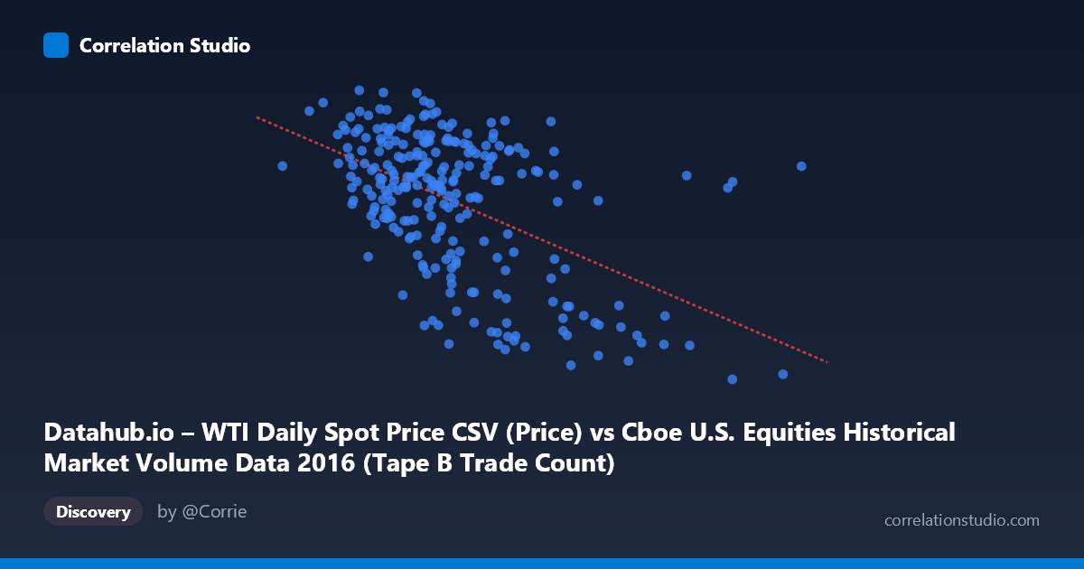
Relationship Overview The scatterplot reveals a moderate negative relationship between WTI daily spot prices (X-axis) and Cboe U.S. Equities Tape B trade counts (Y-axis) across 252 trading days in 2016. As oil prices increase, Tape B trade counts tend to decline, and vice versa. The linear regression equation (y = -3.65e-05x + 54.94) confirms this inverse slope, though the scatter around the regression line is considerable. Visually, the data does not form a tight linear band — there is a broad dispersion, particularly in the mid-range of oil prices, suggesting the relationship is real but far from deterministic.
Correlation Strength and Statistical Significance The Pearson correlation of r = -0.513 indicates a moderate negative association. However, r² = 0.263 tells the more grounded story: only about 26.3% of the variance in Tape B trade counts is explained by WTI prices, meaning roughly 73.7% of the variation is driven by other factors entirely. The 95% confidence interval of [-0.599, -0.416] is meaningfully negative throughout and does not cross zero, lending statistical credibility to the direction of the relationship. With a p-value effectively at 0 across a population of N = 3,622, the correlation is highly unlikely to be a chance artifact. That said, the Granger causality tests yield no significant predictive directionality in either direction (X→Y: F = 0.608, p = 0.436; Y→X: F = 0.977, p = 0.324), meaning that knowing today's oil price does not reliably help predict tomorrow's trade count, and vice versa. This is a critical caveat: the correlation may reflect a shared contemporaneous driver rather than any causal or predictive link.
Notable Patterns and Outliers Several features stand out in the data. There is a visible cluster of high trade-count observations (Y ≈ 45–52) concentrated at lower oil prices (X ≈ 190,000–320,000), consistent with the negative trend. Conversely, lower trade counts (Y ≈ 26–34) appear at higher oil price values (X ≈ 380,000–560,000+), visible in sample points like (381,300, 30.31), (558,190, 29.55), and (467,365, 32.32). A handful of potential outliers exist at the high-X extreme — prices above 500,000 — where trade counts drop sharply, which may represent specific market stress periods or low-liquidity days. Interestingly, the mid-range (X ≈ 280,000–360,000) shows considerable vertical spread in Y (roughly 37 to 51), indicating that at moderate oil prices, equity trading volume is highly variable and poorly predicted by oil alone.
Confounding Factors and Caveats The most significant caveat is the axis labeling ambiguity: the dataset descriptions appear to have the X and Y source labels swapped (WTI price is listed as coming from the Cboe dataset, and Tape B counts from the WTI dataset), which warrants verification before drawing firm conclusions. Beyond this, 2016 was a year of considerable macro volatility — oil recovered from multi-year lows, the U.S. presidential election occurred, and Federal Reserve policy shifts unfolded — all of which independently influenced both oil prices and equity market activity. Seasonality, day-of-week effects, and broader risk-on/risk-off sentiment likely confound this relationship substantially. Tape B specifically covers NYSE American (AMEX) and regional exchange activity, which may have sector-specific sensitivity to energy prices not representative of the broader market. Finally, the Granger test's optimal lag of only 1 period may be too short to capture slower-moving relationships.
Actionable Insights and Further Investigation Despite the lack of Granger causality, the moderate contemporaneous correlation warrants further exploration. Segmenting the data by quarter or by oil price regime (e.g., below vs. above $40/barrel) could reveal whether the relationship strengthens or reverses in specific market conditions. It would be valuable to test longer Granger causality lags (5, 10, 22 trading days) to check for slower transmission mechanisms. Researchers should also control for VIX (volatility index) and broader market volume to isolate whether the oil-Tape B relationship persists independently of general market sentiment. Including energy sector equity flows or Tape A/C data as comparison series would help determine whether this is a sector-specific or market-wide phenomenon. Ultimately, this correlation is a useful exploratory signal, but should not be used for predictive modeling without substantially richer controls.
X dataset: Cboe U.S. Equities Historical Market Volume Data 2016
Y dataset: Datahub.io – WTI Daily Spot Price CSV
Part of experiment: Daily - Cboe U.S. Equities Historical Market Volume Data 2016 vs Datahub.io – WTI Daily Spot Price CSV