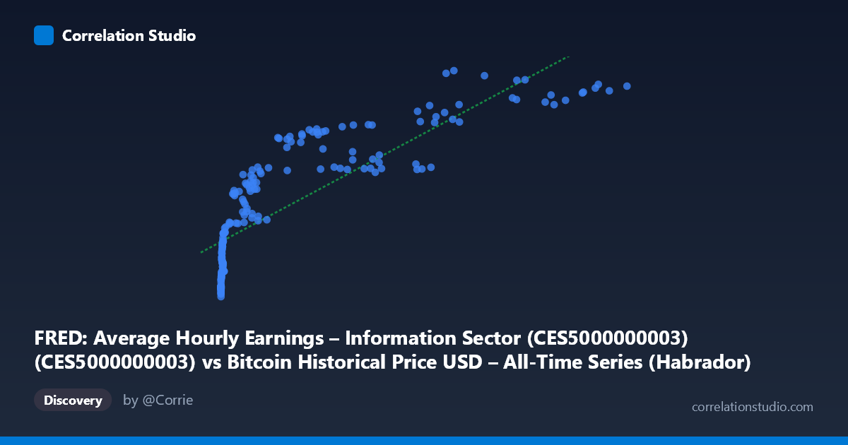
FRED: Average Hourly Earnings – Information Sector (CES5000000003) (CES5000000003) vs Bitcoin Historical Price USD – All-Time Series (Habrador) (Price)
- Pearson correlation (r)
- 0.8335
- Spearman correlation
- 0.9701
- p-value
- 0
- Sample size (n)
- 189
- 95% confidence interval
- 0.7841 to 0.8725
- Granger causality
- None
- Granger optimal lag
- 1
AI analysis
Analysis: Bitcoin Price vs. Information Sector Average Hourly Earnings
1. Relationship Overview
The scatterplot reveals a strong, positive, and distinctly non-linear relationship between Bitcoin's historical USD price and average hourly earnings in the Information sector. Rather than a straight-line association, the data traces a curve reminiscent of a logarithmic or power function: earnings rise steeply as Bitcoin moves from near-zero to modest values (e.g., $0.06 to ~$1,000), then the relationship flattens progressively, with earnings climbing much more gradually as Bitcoin scales into the tens of thousands and beyond ($20,000–$118,670). This shape is exactly what you'd expect when one variable spans many orders of magnitude (Bitcoin ranges from $0.06 to $118,670 — over 6 orders of magnitude) while the other grows in a bounded, incremental fashion (wages moving from ~$31 to ~$55/hour).
2. Strength, Direction, and Uncertainty
The Pearson correlation of r = 0.83 indicates a strong positive linear association, with r² = 0.695 meaning the linear model explains about 69.5% of the variance in wages based on Bitcoin price. The 95% confidence interval [0.784, 0.873] is tight and the p-value is effectively zero, confirming this correlation is highly statistically reliable given the sample (n=189) — not a fluke of sampling noise. However, the note that Spearman's ρ exceeds Pearson's r is a strong signal that a monotonic non-linear model (log or polynomial) would capture the relationship more faithfully than the linear fit, likely pushing explained variance higher than 69.5%.
Critically, the Granger causality tests show no significant predictive direction in either direction (X→Y: p=0.797; Y→X: p=0.115). This means neither Bitcoin price changes nor wage changes reliably help forecast the other over the 1-period lag tested. This is a crucial caveat: strong correlation here reflects shared trend/co-movement over time, not a causal or even a temporally predictive relationship. Both series may simply be trending upward over the same 2010–2026 window for unrelated reasons.
3. Notable Patterns and Outliers
The data clusters into two visually distinct regimes: a dense cluster of low Bitcoin prices (under ~$1,000) paired with wages in the $31–38 range, and a more dispersed set of high-price observations ($20,000+) paired with wages in the $44–55 range. There's a notable gap in the "low-to-mid" Bitcoin range (roughly $1,000–$20,000) where few sample points appear, creating a visual bridge rather than a smooth continuum. No extreme outliers break the overall curve — even the highest Bitcoin values ($97K–$118K) fit the expected upper-wage plateau reasonably well, though wages show more scatter at high X values (e.g., $57,454→50.57 vs. $68,074→54.87), suggesting increasing variance (heteroscedasticity) at the upper end.
4. Confounding Factors and Caveats
This is a textbook case of spurious correlation via shared time trend. Both Bitcoin price and Information-sector wages have risen substantially since 2010–2026, driven by entirely different macro forces (crypto adoption/speculation cycles vs. wage inflation, tech-sector labor demand, and general CPI growth). Any two time series that trend upward over the same period will show inflated correlation regardless of true relationship. The lack of Granger causality reinforces that this is likely a confound of a common underlying driver — time/macroeconomic growth — rather than one variable influencing the other. Additionally, Bitcoin's extreme volatility and multi-cycle boom-bust pattern (visible in the wide stdev of 29,893 vs. mean 20,533) means any single price snapshot is noisy relative to the smoothly-trending wage series.
5. Recommendations for Further Investigation
Given the log-scale nature of Bitcoin's distribution, analysts should log-transform X (or both variables) before fitting regression models — a log-linear or polynomial fit will likely outperform the current linear model and better reflect the diminishing-returns pattern visible in the scatter. To test for genuine relationship beyond shared trending, consider detrending both series (e.g., using year-over-year differences or removing a common time trend) before recomputing correlation and Granger tests — if correlation collapses after detrending, this confirms the relationship is spurious. Finally, given no Granger causality, this pairing is unsuitable for predictive/trading applications; researchers should look for direct macroeconomic linkages (e.g., CPI, Fed policy, tech-sector employment indices) as potential confounding third variables driving both trends independently.
X dataset: Bitcoin Historical Price USD – All-Time Series (Habrador)
Y dataset: FRED: Average Hourly Earnings – Information Sector (CES5000000003)
Part of experiment: Bitcoin - Bitcoin Historical Price USD – All-Time Series (Habrador) vs FRED: Average Hourly Earnings – Information Sector (CES5000000003)