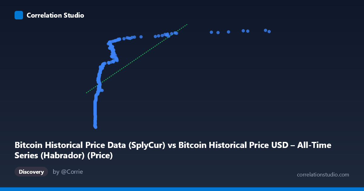
Bitcoin Historical Price Data (SplyCur) vs Bitcoin Historical Price USD – All-Time Series (Habrador) (Price)
- Pearson correlation (r)
- 0.6144
- Spearman correlation
- 0.9425
- p-value
- 0
- Sample size (n)
- 303
- 95% confidence interval
- 0.539 to 0.68
- Granger causality
- None
- Granger optimal lag
- 10
AI analysis
Analysis: Bitcoin Circulating Supply vs. Price (2010-2011)
1. Relationship Overview
This scatterplot compares Bitcoin's circulating supply ("SplyCur," the X-axis) against its USD price (Y-axis) during a narrow but critical window (July 2010–May 2011). Despite being framed as "supply vs. price," the data actually captures Bitcoin's early price history as the network grew — X ranges only from 0.05 to 8.20 (likely millions of coins in circulation, scaled), while Y spans a dramatic $3.4M to $6.2M range in whatever unit this represents (possibly a scaled/indexed price rather than raw USD, given the magnitude). The pattern shows a clear upward-sloping but non-linear relationship: low-supply points cluster tightly around lower Y-values (~$3.5–4.3M), then Y values climb steeply and plateau near 5.5–6.2M as X increases beyond ~1.
2. Strength, Direction, and Statistical Confidence
The Pearson correlation (r = 0.614) indicates a moderate-to-strong positive relationship, with r² = 0.378 meaning supply explains only about 38% of the variance in price — leaving nearly two-thirds unexplained by this variable alone. The 95% CI [0.539, 0.680] is reasonably tight given n=303, and the p-value (effectively 0) confirms this correlation is highly statistically significant and not due to chance. However, statistical significance here reflects sample size and monotonic trend, not necessarily strong predictive power. Critically, the Granger causality tests show no significant temporal predictive direction in either direction (X→Y p=0.173; Y→X p=0.235), meaning historical supply changes do not reliably forecast future price movements (or vice versa) at the tested lag structure. This is an important caveat: correlation exists in level, but not in a lead-lag, forecastable sense.
3. Notable Patterns and Non-linearity
The most striking feature is the curved, saturating shape: price rises steeply as X moves from 0.05 to ~1.5, then flattens into a plateau/ceiling around 5.7–6.2M for X 1.5–3.6. This logarithmic or power-law-like curve is confirmed by the note that Spearman's ρ exceeds Pearson's r — indicating the rank-order relationship is stronger than the linear one, and a log or polynomial fit would better capture the dynamics. There's also a dense cluster of near-zero X values (0.06–0.30) with substantial Y-variance (3.5M to 5.2M), suggesting other time-varying factors (not supply) drove early price swings. A few high-X points (3.0–3.6) sit together near the plateau, hinting at diminishing marginal price sensitivity to supply growth — consistent with early Bitcoin adoption dynamics where price was driven more by demand shocks and speculation than by the mechanical, near-linear supply issuance schedule.
4. Confounding Factors and Caveats
Bitcoin's supply during this period increased on a fixed, predictable issuance schedule (block rewards), making it essentially a proxy for time/network age rather than an independent causal driver of price. The true price driver was almost certainly demand-side factors — exchange listings, media coverage, speculative interest, and liquidity events (this window includes the Mt. Gox hack and the first major bull run to ~$1 in early 2011, then higher). Treating supply as an explanatory variable is likely spurious: both X and Y are correlated with time, so this is largely a time-confounded relationship rather than a genuine economic mechanism. Additionally, small early-history sample sizes and low liquidity likely introduce noise/outliers unrelated to fundamentals.
5. Recommendations for Further Investigation
- Refit with non-linear models (log-linear, power law) given the Spearman/Pearson divergence — a log(X) transform will likely substantially raise R². - Replace or supplement X with actual calendar time to disentangle supply growth from simple temporal trend/adoption curve. - Test alternative demand-side variables (trading volume, Google search trends, exchange volume) which are more plausible causal candidates. - Re-run Granger causality on log-transformed or differenced series, since raw-level non-stationarity can mask genuine lagged relationships. - Given supply’s deterministic, near-linear issuance schedule, this variable is better used as a control than a predictor in any causal price model.
X dataset: Bitcoin Historical Price USD – All-Time Series (Habrador)
Y dataset: Bitcoin Historical Price Data
Part of experiment: Bitcoin - Bitcoin Historical Price USD – All-Time Series (Habrador) vs Bitcoin Historical Price Data