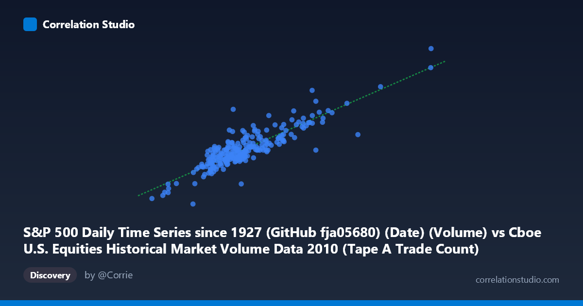
S&P 500 Daily Time Series since 1927 (GitHub fja05680) (Date) (Volume) vs Cboe U.S. Equities Historical Market Volume Data 2010 (Tape A Trade Count)
- Pearson correlation (r)
- 0.8736
- Spearman correlation
- 0.8051
- p-value
- 0
- Sample size (n)
- 252
- 95% confidence interval
- 0.8409 to 0.9001
- Granger causality
- None
- Granger optimal lag
- 10
AI analysis
Scatterplot Analysis: S&P 500 Daily Volume vs. Cboe Tape A Trade Count (2010)
Relationship Overview The scatterplot reveals a strong positive linear relationship between S&P 500 daily trading volume and Cboe Tape A trade count across the 2010 trading year. As daily volume increases, the number of individual trades recorded on Tape A rises proportionally, which is broadly intuitive — higher volume days tend to involve more discrete transactions. The linear regression model (y = 2584.1x + 1.167×10⁹) captures this trend well, with the data points clustering reasonably tightly around the regression line across most of the range, suggesting the relationship is consistent rather than episodic.
Correlation Strength and Statistical Significance The Pearson correlation of r = 0.8736 indicates a strong positive association, and the R² of 0.7633 means that approximately 76.3% of the variance in Tape A trade count is explained by daily S&P 500 volume — a substantial explanatory share. The 95% confidence interval of [0.8409, 0.9001] is notably narrow, reflecting the large paired sample (n = 252, drawn from a population of N = 3,302), and the p-value of effectively zero confirms this is not a chance finding. However, the remaining ~23.7% of unexplained variance is non-trivial and warrants attention. Critically, the Granger causality tests reveal no statistically significant predictive directionality in either direction (X→Y: F = 1.72, p = 0.077; Y→X: F = 0.98, p = 0.463). Neither series meaningfully predicts the other temporally at the optimal 10-period lag, suggesting the correlation reflects contemporaneous co-movement driven by shared underlying forces rather than one variable leading the other.
Notable Patterns, Clusters, and Outliers The data broadly forms a coherent linear band, but several features stand out. A high-leverage outlier near (3,216,587 volume, 9.47 billion trade count) sits well above the main cluster and likely represents an exceptional market event day in 2010 — possibly tied to the May 6th Flash Crash or a major macro announcement. At the lower end, a point near (796,428 volume, 1.29 billion trade count) is notably depressed on both axes, suggesting an unusually quiet session. Additionally, a point at approximately (2,474,888 volume, 5.45 billion trade count) appears as a moderate outlier in a different direction — high volume but relatively low trade count — implying a day with large average trade sizes, potentially dominated by block trades or institutional activity rather than high-frequency retail fragmentation. The bulk of observations cluster between 800K–1.8M volume and 3–6.5 billion trade count, forming the core of the relationship.
Confounding Factors and Interpretive Caveats Several important caveats apply. First, both variables are likely driven by common third factors — market volatility (VIX), earnings seasons, macroeconomic releases, or Federal Reserve announcements — which would inflate the observed correlation without implying a direct structural link. Second, the dataset covers only calendar year 2010, a specific post-crisis recovery period; the relationship may not generalize to other market regimes (e.g., low-volatility 2017 or crisis-period 2020). Third, the axis labels contain a subtle dataset cross-referencing quirk (the S&P 500 GitHub dataset's volume column is paired with the Cboe trade count), so users should verify that volume figures are consistently defined (shares vs. notional value vs. contract count). Finally, the absence of Granger causality at a 10-period lag does not rule out contemporaneous or very short-lag relationships that this test structure may not capture.
Actionable Insights and Further Investigation Practitioners examining market microstructure should investigate the high-volume outliers individually to determine whether they skew the regression intercept meaningfully. Incorporating a volatility measure (e.g., realized volatility or VIX) as a covariate would help disentangle whether volume→trade count relationships hold after controlling for market stress. It would also be valuable to extend the time series beyond 2010 to test whether the R² and slope are stable across different market cycles — a degrading R² over time could signal structural changes in trading fragmentation or algorithmic activity. Finally, segmenting the data by day-of-week or proximity to major announcements could reveal whether the unexplained 23.7% variance is systematically distributed, which would be actionable for execution timing strategies.
X dataset: Cboe U.S. Equities Historical Market Volume Data 2010
Y dataset: S&P 500 Daily Time Series since 1927 (GitHub fja05680) (Date)
Part of experiment: Daily - Cboe U.S. Equities Historical Market Volume Data 2010 vs S&P 500 Daily Time Series since 1927 (GitHub fja05680) (Date)