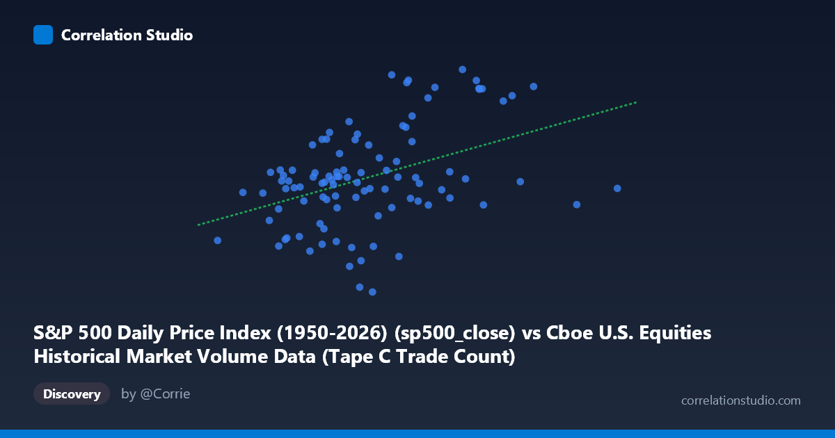
S&P 500 Daily Price Index (1950-2026) (sp500_close) vs Cboe U.S. Equities Historical Market Volume Data (Tape C Trade Count)
- Pearson correlation (r)
- 0.4154
- Spearman correlation
- 0.347
- p-value
- 0.000021
- Sample size (n)
- 98
- 95% confidence interval
- 0.2364 to 0.567
- Granger causality
- None
- Granger optimal lag
- 10
AI analysis
Scatterplot Analysis: S&P 500 Price vs. Cboe Tape C Trade Count
Overview of the Relationship
The scatterplot reveals a modest positive relationship between the S&P 500 Daily Price Index and the Cboe U.S. Equities Tape C Trade Count over the period from January 2 to May 22, 2026. As the S&P 500 price rises, Tape C trade counts tend to increase as well, consistent with the fitted regression line (y = 0.000330x + 5868.82). However, the relationship is far from tight — there is considerable vertical scatter at nearly every level of X, indicating that many other factors beyond price level are driving daily trade activity. The data spans a meaningful but relatively short five-month window, which limits generalizability but provides a contemporaneous snapshot of market microstructure dynamics.
Correlation Strength, Significance, and Causality
The Pearson correlation of r = 0.4154 indicates a weak-to-moderate positive association, but the explanatory power is limited: r² = 0.1725, meaning only about 17.3% of the variance in Tape C trade counts is explained by the S&P 500 price level. The remaining ~83% of variation is attributable to factors outside this model. The 95% confidence interval for r of [0.2364, 0.5670] is moderately wide, reflecting meaningful uncertainty around the true population correlation, though the interval excludes zero entirely. The p-value of 2.11 × 10⁻⁵ confirms that the correlation is statistically significant at conventional thresholds (p < 0.001), so the positive association is unlikely to be a sampling artifact given n = 98. Crucially, however, the Granger causality tests find no significant predictive directionality in either direction — neither X→Y (F = 0.66, p = 0.757) nor Y→X (F = 1.10, p = 0.373) reaches significance at a 10-period lag. This means that while the two variables are contemporaneously correlated, past values of one do not reliably predict future values of the other, severely limiting any trading or forecasting utility of this relationship in a temporal context.
Notable Patterns, Clusters, and Outliers
Several features stand out in the data. There appears to be a cluster of observations in the X range of roughly 2,850,000–3,200,000 where Y values span a wide range (~6,350–7,175), suggesting high dispersion at moderate price levels. At higher X values (above ~3,600,000), Y values tend to concentrate in the upper register (~7,300–7,500), pulling the regression line upward and contributing disproportionately to the positive slope. A few points appear to be potential outliers: notably one observation near (3,205,940; 6,368.85), another near (3,262,293; 6,343.72), and the extreme X-axis point at approximately (4,341,729; 6,882.72), which is a clear leverage point. The high-X, moderate-Y outlier at ~4.34M could meaningfully influence the regression slope and warrants separate examination. There is also a noticeable lower boundary of Y values around 6,343–6,400 suggesting a possible floor in trade counts during this period.
Confounding Factors and Interpretive Caveats
Several important caveats apply. First, both variables are likely driven by shared macroeconomic forces — volatility regimes, earnings seasons, Federal Reserve policy announcements, and broader risk-on/risk-off sentiment — which can create spurious or inflated correlations without implying any direct mechanism. Second, Tape C specifically captures Nasdaq-listed securities, so the relationship may partly reflect the outsized weight of mega-cap tech stocks in both the S&P 500 price index and Nasdaq trading volume, rather than a generalizable market-wide phenomenon. Third, using price level rather than returns or volatility is methodologically significant — price is non-stationary, which can produce misleading correlations over time (a classic spurious regression risk). Fourth, with only 98 paired observations drawn from a population of 1,980, sampling variability remains a concern even with a significant p-value. Finally, the optimal lag of 10 periods in the Granger test is relatively long; shorter lags were presumably tested and also found non-significant, but sensitivity across all lag choices should be verified.
Actionable Insights and Further Investigation
Given the moderate correlation, limited explanatory power, and absence of Granger causality, this relationship should not be used directly as a predictive trading signal. However, several investigative paths are worth pursuing. Analysts should consider replacing the price level with daily log returns or realized volatility as the X variable, as volatility is a far more theoretically grounded driver of trade count activity. Segmenting the data by VIX regime or earnings calendar periods could reveal whether the correlation strengthens under specific market conditions. Investigating the outlier observations — particularly the extreme high-X point and the very low-Y cluster — could uncover data quality issues or regime changes deserving separate modeling. Additionally, running this analysis across longer historical windows (the full 2009–2026 dataset is available) would test whether this correlation is structurally stable or specific to early 2026 market conditions. Finally, a multivariate model incorporating volume, volatility, and macro indicators alongside price would likely explain substantially more of the Tape C trade count variance than this bivariate framework.
X dataset: Cboe U.S. Equities Historical Market Volume Data
Y dataset: S&P 500 Daily Price Index (1950-2026)
Part of experiment: Daily - Cboe U.S. Equities Historical Market Volume Data vs S&P 500 Daily Price Index (1950-2026)