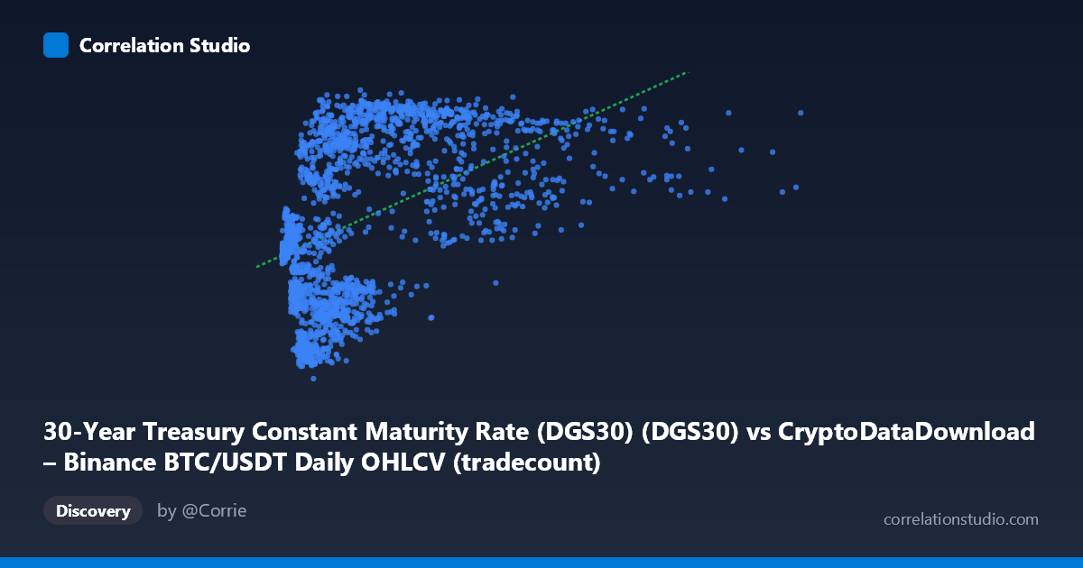
30-Year Treasury Constant Maturity Rate (DGS30) (DGS30) vs CryptoDataDownload – Binance BTC/USDT Daily OHLCV (tradecount)
- Pearson correlation (r)
- 0.4754
- Spearman correlation
- 0.4881
- p-value
- 0
- Sample size (n)
- 2197
- 95% confidence interval
- 0.4424 to 0.5071
- Granger causality
- None
- Granger optimal lag
- 1
- Time coverage
- 2017-08-17 to 2026-06-25
- Recomputed on refreshed data
- 2026-10-24 (r was 0.4754)
AI analysis
Analysis: BTC/USDT Trading Data vs. 30-Year Treasury Yield
Note on axis labeling: The axis labels appear swapped/mismatched in the metadata—X is described as DGS30 (Treasury rate) but ranges into the millions (3,070 to 15,364,010), which is characteristic of trade count data, while Y ranges from 0.99 to 5.18, consistent with a Treasury yield in percentage terms. The analysis below treats X as the large-magnitude variable (likely BTC/USDT trade count or volume) and Y as the Treasury yield (DGS30), based on the actual data ranges.
1. What the Visualization Reveals The scatterplot shows a moderate positive association: as the X variable (trade count/volume) increases, Y (the 30-year yield) tends to rise as well, though with substantial scatter. The relationship is not tight — points are widely dispersed around the regression line, particularly at low X values where Y ranges anywhere from ~1.3 to ~4.9, indicating that low trading activity days occur across the full spectrum of yield environments.
2. Strength, Direction, and Statistical Confidence The correlation coefficient (r = 0.475) indicates a moderate positive relationship. With r² = 0.226, only 22.6% of the variance in Y is explained by X — meaning roughly 77% of the variation in yields is driven by other factors entirely unrelated to this X variable. The 95% CI [0.442, 0.507] is fairly narrow, and the p-value of ~0 confirms this correlation is statistically robust and not due to chance, aided by the large sample (n=2,197). However, statistical significance here reflects sample size more than practical predictive power — a moderate r with n2000 is easy to detect but still leaves most variance unexplained. Critically, the Granger causality tests show no significant predictive direction in either direction (X→Y: p=0.474; Y→X: p=0.746). This means neither variable's past values help forecast the other's future values — the correlation is likely contemporaneous/coincidental (e.g., both trending over the 2017–2026 period) rather than causal or lead-lag in nature.
3. Notable Patterns and Outliers The data shows a fan/wedge shape: at low X values (under ~2M), Y spans almost the entire observed range (1.3–4.9), while at higher X values (5M), Y clusters more narrowly in the 3.2–4.9 band. This heteroscedasticity suggests the relationship may not be strictly linear — possibly logarithmic or threshold-based, where high trading activity coincides with a narrower, higher-yield regime. A few high-X outliers (8.8M, 6.8M) sit at moderate Y values (~3.2–3.65), slightly below the trend, hinting at diminishing returns rather than a straight-line relationship. There's also a visible cluster of low-X, low-Y points (X<1M, Y<2.5) representing a distinct regime, possibly an early time period.
4. Confounding Factors and Caveats Both series are time-ordered macro/market variables spanning 2017–2026, a period during which both Treasury yields and crypto trading volumes independently trended upward (yields rose from near-zero to multi-year highs post-2022; crypto trading activity grew with market maturation). This shared temporal trend is a classic spurious correlation setup — both variables may simply be correlated with time/date itself rather than with each other causally. The mismatched axis descriptions also raise data-quality concerns that should be resolved before drawing firm conclusions. Additionally, daily trade count/volume is a noisy, activity-driven metric while DGS30 is a slow-moving macro rate — their natural time scales differ substantially, complicating any causal interpretation.
5. Recommendations for Further Investigation 1. Clarify and correct axis labels/data mapping before further analysis — verify which dataset actually populates X vs Y. 2. De-trend both series (e.g., via differencing or detrending against date) and re-run correlation to check if the relationship survives after removing shared time trends — this is essential given the Granger non-causality finding. 3. Segment by regime (e.g., pre/post-2022 rate hikes) to test whether the correlation is stable or driven by a specific sub-period. 4. Explore non-linear fits (log-X transformation) given the fan-shaped scatter, which may better capture the relationship than the current linear model (R²=0.226). 5. Given the lack of Granger causality, avoid using either series to forecast the other; instead, treat the correlation as descriptive/contemporaneous only, not predictive.
X dataset: CryptoDataDownload – Binance BTC/USDT Daily OHLCV
Y dataset: 30-Year Treasury Constant Maturity Rate (DGS30)
Part of experiment: Bitcoin - CryptoDataDownload – Binance BTC/USDT Daily OHLCV vs 30-Year Treasury Constant Maturity Rate (DGS30)