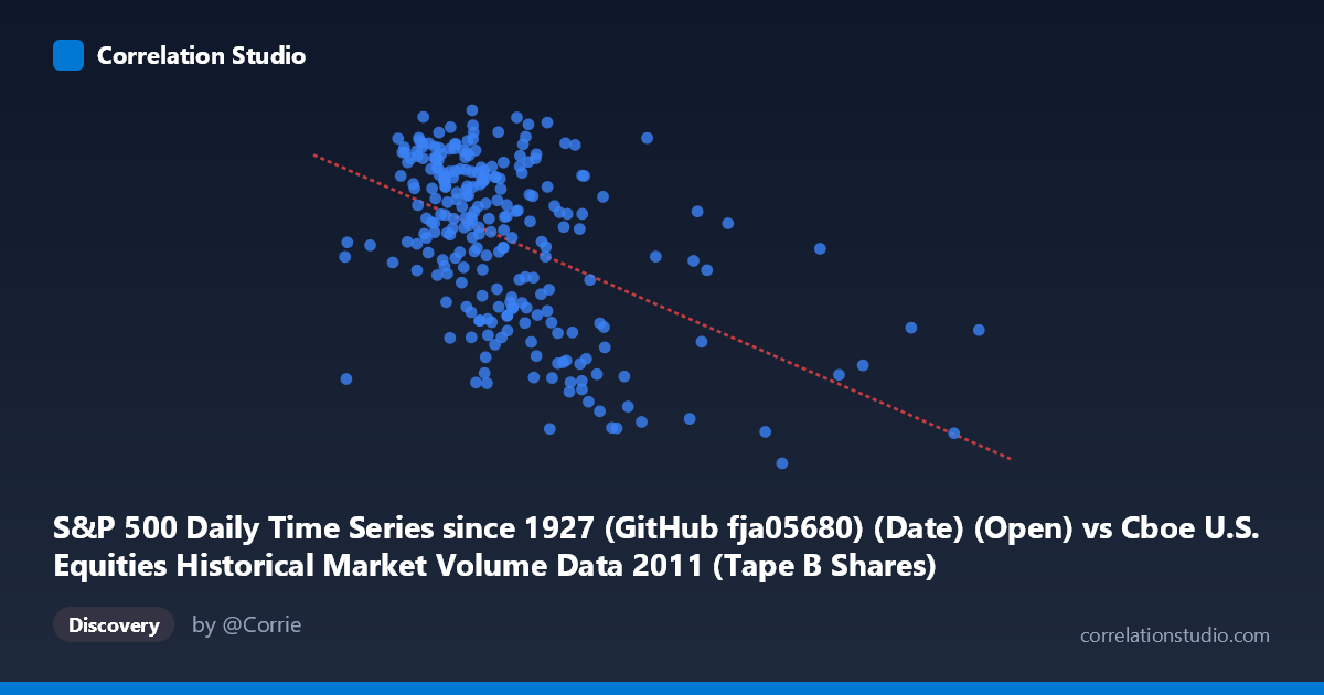
S&P 500 Daily Time Series since 1927 (GitHub fja05680) (Date) (Open) vs Cboe U.S. Equities Historical Market Volume Data 2011 (Tape B Shares)
- Pearson correlation (r)
- -0.493
- Spearman correlation
- -0.4729
- p-value
- 0
- Sample size (n)
- 252
- 95% confidence interval
- -0.5811 to -0.3934
- Granger causality
- None
- Granger optimal lag
- 1
AI analysis
Analysis: S&P 500 Open Price vs. Cboe Tape B Shares Volume (2011)
Relationship Overview The scatterplot reveals a moderate negative relationship between S&P 500 daily open prices and Cboe Tape B shares volume throughout 2011. As the S&P 500 open price increases, Tape B share volume tends to decrease, and vice versa. This inverse pattern is visually apparent across the data cloud, though with considerable scatter. The linear regression equation (y = -9.36e-7x + 1359.48) quantifies this: for every ~1 million unit increase in the S&P 500 open value, Tape B volume declines by roughly 0.94 units, anchored around a baseline of approximately 1,359 shares.
Correlation Strength and Statistical Significance The Pearson correlation of r = -0.493 indicates a moderate negative association, but the more meaningful metric is r² = 0.243 — meaning S&P 500 open prices explain only 24.3% of the variance in Tape B shares volume, leaving roughly 75.7% attributable to other factors. The 95% confidence interval of [-0.581, -0.393] is entirely negative and does not cross zero, confirming directional consistency. With a p-value of effectively 0 and a sample of 252 paired observations drawn from a population of 3,780, the correlation is highly statistically significant and unlikely to be a chance artifact. However, the Granger causality results are striking in their null findings: neither direction (X→Y: F=0.0022, p=0.963; Y→X: F=0.0001, p=0.991) shows any meaningful temporal predictive power. This means that while a contemporaneous correlation exists, past S&P 500 prices do not help predict future Tape B volume, and vice versa — a critical distinction between association and predictive causation.
Patterns, Clusters, and Outliers Several notable features emerge from the sample points. There is a visible cluster of high-volume observations (Y ~1,300–1,365) concentrated at lower X values (roughly 60–100 million range), consistent with elevated retail and institutional trading activity during market stress periods when prices were depressed — characteristic of 2011's August debt-ceiling crisis and European sovereign debt turmoil. Conversely, high-X outliers (e.g., ~189.7M, ~176.5M, ~169.1M) are associated with notably lower Tape B volumes (~1,121–1,280), suggesting that elevated price environments coincided with reduced Tape B activity. The spread is widest in the mid-X range (~80–130M), indicating heteroscedasticity — the relationship is less predictable at moderate price levels than at extremes.
Confounding Factors and Caveats Several important caveats apply. First, Tape B represents only one market tier (NYSE American and regional exchange-listed securities), so its volume dynamics may reflect competitive routing decisions, maker-taker fee structures, or regulatory changes rather than broad market sentiment. Second, the inverse relationship likely reflects a risk-off/risk-on dynamic: lower S&P prices in 2011 often coincided with volatility spikes (VIX surges), which historically drive higher share turnover — but this is a confound mediated by volatility, not price per se. Third, the data covers only a single calendar year (2011), a particularly turbulent period; the relationship may not generalize to other market regimes. Fourth, using Open price as a proxy for market level introduces intraday timing ambiguity relative to daily volume measurements.
Actionable Insights and Further Investigation Given that the correlation is statistically robust but explains less than a quarter of variance and carries no Granger-causal signal, practitioners should avoid using S&P 500 open levels as a standalone predictor of Tape B volume for trading or liquidity models. More productive next steps would include: (1) incorporating realized volatility (VIX or intraday range) as a mediating variable, which likely explains a substantial portion of the residual 75.7% variance; (2) testing whether the relationship is non-linear (e.g., threshold effects below key price levels like the August 2011 crash trough); (3) extending the analysis across multiple years to assess regime stability; and (4) decomposing Tape B volume by trade size to distinguish institutional block activity from retail order flow, which may respond differently to price-level changes.
X dataset: Cboe U.S. Equities Historical Market Volume Data 2011
Y dataset: S&P 500 Daily Time Series since 1927 (GitHub fja05680) (Date)
Part of experiment: Daily - Cboe U.S. Equities Historical Market Volume Data 2011 vs S&P 500 Daily Time Series since 1927 (GitHub fja05680) (Date)