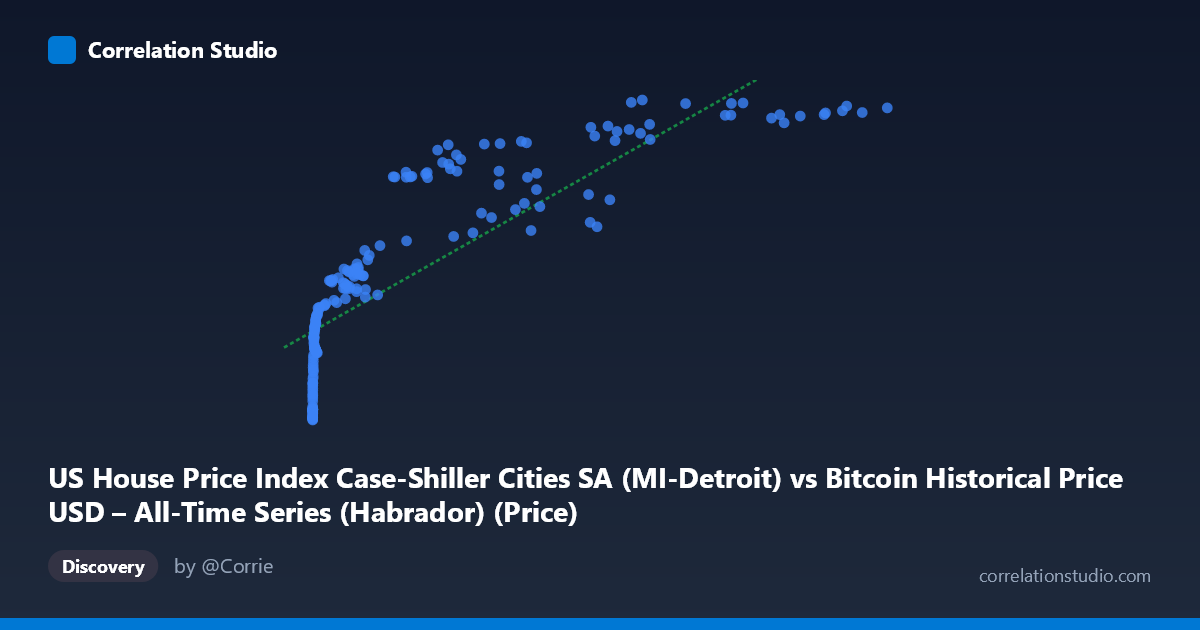
US House Price Index Case-Shiller Cities SA (MI-Detroit) vs Bitcoin Historical Price USD – All-Time Series (Habrador) (Price)
- Pearson correlation (r)
- 0.8438
- Spearman correlation
- 0.9733
- p-value
- 0
- Sample size (n)
- 189
- 95% confidence interval
- 0.7971 to 0.8805
- Granger causality
- None
- Granger optimal lag
- 1
- Time coverage
- 2010-08-01 to 2026-04-01
- Recomputed on refreshed data
- 2026-10-22 (r was 0.8362)
AI analysis
Analysis: Bitcoin Price vs. Detroit Case-Shiller Home Price Index
1. Relationship Overview
The scatterplot shows a strong positive association between Bitcoin's historical USD price and the Detroit Case-Shiller Home Price Index, but the relationship is distinctly non-linear. At low Bitcoin prices (under ~$1,000), the index values cluster tightly between 67–115, showing rapid index growth even as Bitcoin moves from fractions of a cent to a few dollars. As Bitcoin climbs into the thousands and tens of thousands, the index growth decelerates and plateaus in the 180–200 range. This curve shape — steep initial rise followed by flattening — is characteristic of a logarithmic relationship, which is confirmed by the fact that Spearman's rank correlation exceeds Pearson's r.
2. Strength, Direction, and Causality
The Pearson correlation (r = 0.836, r² = 0.699) indicates a strong positive linear relationship, with the linear model explaining roughly 70% of the variance in the home price index. The 95% confidence interval [0.787, 0.875] is tight and does not cross zero, and the p-value of effectively 0 confirms this correlation is highly statistically significant — not a chance artifact of the 186-point sample. However, statistical significance and strength of correlation do not imply causation. The Granger causality tests are decisive here: neither direction shows significant predictive power (Bitcoin→Housing: p=0.40; Housing→Bitcoin: p=0.12). This means neither series' past values help forecast the other's future movements in a time-series sense — the strong contemporaneous correlation is likely driven by both variables trending upward over the same historical period (2010–2026) rather than one causing the other.
3. Notable Patterns and Outliers
Several features stand out: (a) a dense cluster of low-value points (X < 100, Y < 90) representing Bitcoin's earliest years, which anchor the low end of the curve; (b) a "middle" cluster (X: 1,000–20,000; Y: 105–170) representing the 2017–2020 era; and (c) a high-value cluster (X 50,000, Y 180) reflecting recent years where the housing index has largely saturated near its ceiling (~190–200) while Bitcoin continues to swing widely ($57K–$118K), showing heteroscedasticity — variance in X is much larger than in Y at high values. This flattening at the top is the key non-linear signature: the housing index is bounded/slow-moving while Bitcoin is highly volatile, so a linear fit understates the true fit quality captured by a log or power-law model.
4. Confounding Factors and Caveats
The most important caveat is that both series are independently trending upward over the same 15-year window — Bitcoin due to adoption/speculation cycles, and the housing index due to broad U.S. macroeconomic inflation, low interest rates (2010s), and post-pandemic housing demand. This is a classic case of spurious correlation via shared time trend: two unrelated non-stationary time series will often show high correlation simply because both increase over time. The Granger test results reinforce this — there's no evidence of genuine lead-lag predictive relationship. Additionally, comparing a single city's housing index (Detroit) to a global speculative asset (Bitcoin) lacks a clear economic mechanism; any relationship is likely mediated by macro factors like monetary policy, inflation expectations, or overall risk appetite rather than direct interaction.
5. Actionable Insights
For more rigorous analysis: (1) Detrend or difference both series (e.g., use year-over-year % changes) before computing correlation to test whether the relationship survives after removing shared trend — this would better isolate genuine co-movement from spurious trend correlation. (2) Fit a logarithmic or power model (e.g., Y = a·ln(X) + b) given the non-linear curve shape and Spearman/Pearson discrepancy, which should improve explained variance. (3) Test cointegration (e.g., Engle-Granger) rather than relying on simple correlation, since both series appear non-stationary. (4) Compare against a broader housing index (e.g., national Case-Shiller) or other risk assets (S&P 500) to determine if Bitcoin's correlation with Detroit housing is unique or simply reflects a general "risk-on" macro correlation with all appreciating asset classes over this period.
X dataset: Bitcoin Historical Price USD – All-Time Series (Habrador)
Y dataset: US House Price Index Case-Shiller Cities SA
Part of experiment: Bitcoin - Bitcoin Historical Price USD – All-Time Series (Habrador) vs US House Price Index Case-Shiller Cities SA