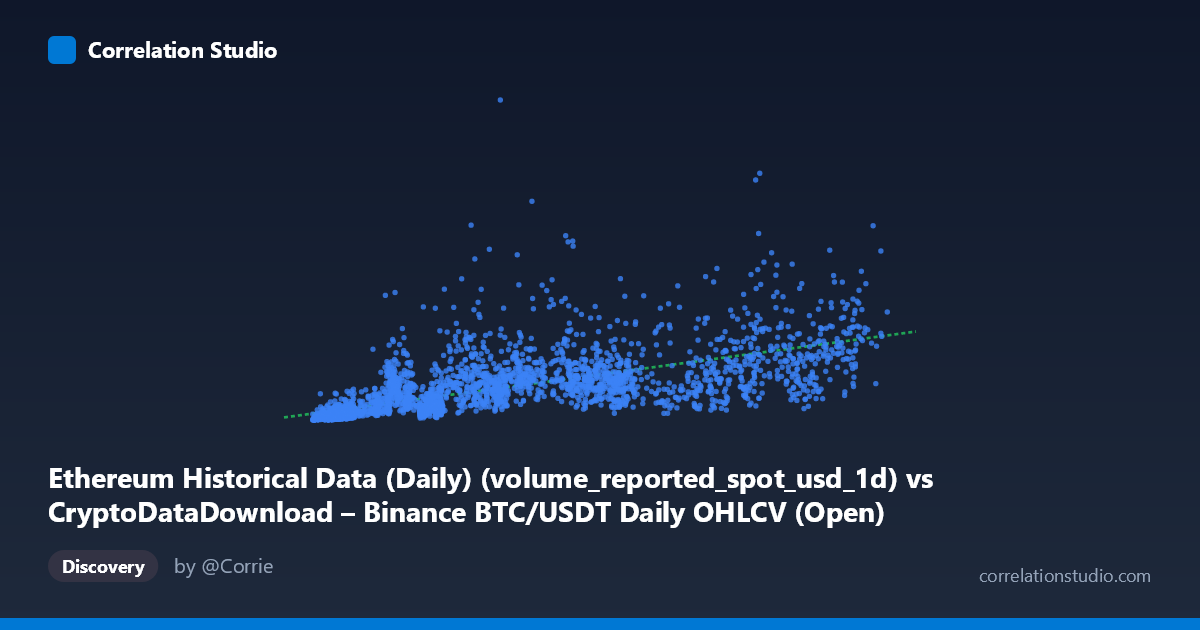
Ethereum Historical Data (Daily) (volume_reported_spot_usd_1d) vs CryptoDataDownload – Binance BTC/USDT Daily OHLCV (Open)
- Pearson correlation (r)
- 0.6766
- Spearman correlation
- 0.8424
- p-value
- 0
- Sample size (n)
- 3191
- 95% confidence interval
- 0.6573 to 0.6949
- Granger causality
- Y → X
- Granger optimal lag
- 10
AI analysis
Analysis: Volume/Price Relationship (Mislabeled Cross-Asset Data)
Important caveat first: The column labels here are internally inconsistent — the X-axis is described as "volumereportedspotusd1d" for BTC/USDT, while the Y-axis is described as an "Open" price field but attributed to an Ethereum dataset described as "network and market metrics." Given the magnitudes (X: ~3K–125K; Y: ~$100M–$53B), this looks like X is a daily trading volume-like metric and Y is a much larger dollar-denominated market metric (possibly total market cap, cumulative volume, or aggregated on-chain value flow) rather than a simple per-coin price. The analysis below treats the data at face value as "X = a volume/activity metric" and "Y = a large-scale dollar value metric," but any conclusions should be revisited once the column identities are clarified.
1. What the Visualization Reveals The scatterplot shows a clear positive, monotonic relationship: as X increases, Y tends to increase as well, but the relationship is not tightly linear. Points fan out increasingly at higher X values (heteroscedasticity), and several high-Y outliers appear at moderate X values (e.g., X≈40,680 → Y≈$14.6B; X≈57,037 → Y≈$15.0B), suggesting the relationship may follow a curved (power-law or logarithmic) rather than straight-line path — consistent with the note that Spearman's ρ exceeds Pearson's r.
2. Strength, Direction, and Statistical Confidence The Pearson correlation (r = 0.677) indicates a moderately strong positive linear relationship, with r² = 0.458 meaning only about 46% of the variance in Y is explained by X in a linear model — leaving more than half of Y's variability unaccounted for by X alone. The 95% CI [0.657, 0.695] is narrow and does not cross zero, and the p-value is effectively 0, so we can be confident the correlation is real and not a sampling artifact, even though it is far from a deterministic relationship. Critically, the Granger causality test points to Y predicting X, not the reverse (Y→X: F=2.43, p=0.0069; X→Y: F=1.26, p=0.245). This means past values of Y have statistically significant predictive power for future X, while X shows no such predictive power for Y — the opposite of what one might assume if X were "volume" driving "price/value."
3. Notable Patterns and Outliers - Non-linear curvature: Several low-to-mid X points show disproportionately high Y (e.g., X≈35,546 → Y≈$7.7B; X≈40,680 → Y≈$14.6B), while some higher-X points show comparatively modest Y (X≈89,995 → Y≈$3.07B; X≈76,346 → Y≈$3.08B) — this scatter pattern is inconsistent with pure linearity and supports fitting a log or power model instead. - Heteroscedasticity: Variance in Y grows substantially as X increases, a classic sign that a log-log or log-linear transformation would stabilize the relationship and likely improve fit. - Low-X cluster: Many low-X points (X<10,000) cluster tightly with lower Y values, forming a dense, well-behaved region, while the sparser high-X tail drives most of the scatter/uncertainty.
4. Confounding Factors and Caveats Both series likely share a common underlying driver — overall crypto market cycles (bull/bear regimes), macro liquidity conditions, and BTC/ETH price co-movement — which would inflate the correlation without implying direct causation between the specific metrics measured. Because both variables are time series spanning 2017–2026, they are almost certainly non-stationary and autocorrelated; naive Pearson/Granger tests on levels (rather than returns or differenced/detrended series) can produce spurious correlation and misleading causality signals. The metric mismatch (per-transaction volume vs. an aggregate multi-billion-dollar figure) also raises the possibility that Y is a cumulative or market-wide quantity, which would mechanically trend with time alongside X, inflating r without genuine mechanistic linkage.
5. Suggestions for Further Investigation 1. Clarify data provenance — confirm what X and Y actually represent (the labels are contradictory) before drawing economic conclusions. 2. Re-fit on log-transformed variables (log(X), log(Y)) or test polynomial fits, since Spearman Pearson and the visual fan-shape both suggest a non-linear (likely power-law) relationship would raise explained variance well above 45.8%. 3. Test stationarity and use returns/differences for the Granger causality analysis to rule out spurious causality from shared trends; consider a VECM if the series are cointegrated. 4. Control for time/market regime (e.g., include a bull/bear dummy or BTC price as a covariate) to isolate whether the X–Y link is direct or mediated by broader market conditions. 5. Investigate the Y→X causal signal further — if confirmed robust, this counterintuitive direction (a value metric predicting a volume metric) could have practical trading/forecasting value and merits a dedicated lagged-regression or VAR impulse-response study.
X dataset: CryptoDataDownload – Binance BTC/USDT Daily OHLCV
Y dataset: Ethereum Historical Data (Daily)
Part of experiment: Bitcoin - CryptoDataDownload – Binance BTC/USDT Daily OHLCV vs Ethereum Historical Data (Daily)