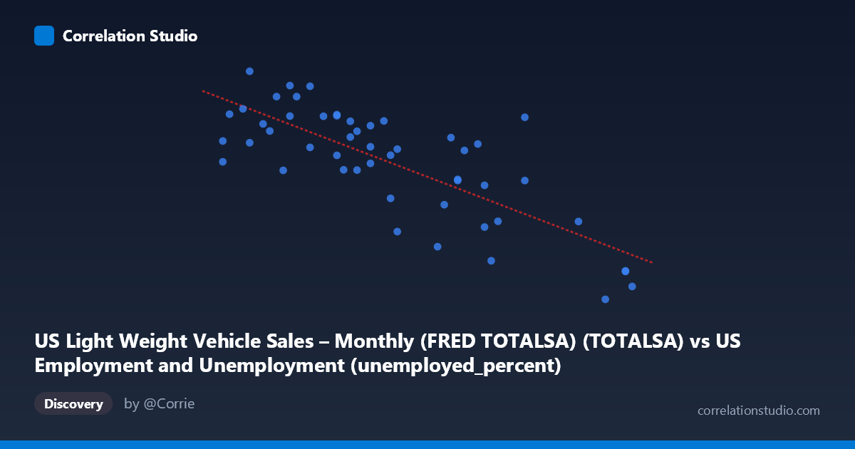
US Light Weight Vehicle Sales – Monthly (FRED TOTALSA) (TOTALSA) vs US Employment and Unemployment (unemployed_percent)
- Pearson correlation (r)
- -0.7725
- Spearman correlation
- -0.7178
- p-value
- 0
- Sample size (n)
- 50
- 95% confidence interval
- -0.8649 to -0.6295
- Granger causality
- None
- Granger optimal lag
- 1
- Time coverage
- 1976-01-01 to 2025-01-01
- Recomputed on refreshed data
- 2026-10-07 (r was -0.7609)
AI analysis
Analysis: US Light Vehicle Sales vs. Unemployment Rate
Relationship Overview
The scatterplot reveals a moderately strong negative relationship between US light weight vehicle sales (X) and the unemployment rate (Y), meaning that as vehicle sales increase, unemployment tends to decrease, and vice versa. This is intuitively coherent: periods of economic expansion typically feature both robust consumer spending on big-ticket items like automobiles and tighter labor markets. The linear regression equation (y = -0.974x + 21.00) suggests that for every additional million units in annualized vehicle sales, the unemployment rate falls by approximately 0.97 percentage points — nearly a one-for-one trade-off in scale. The data span nearly five decades (1976–2025), capturing multiple full business cycles, which adds meaningful breadth to this observed pattern.
Correlation Strength and Statistical Significance
The Pearson correlation of r = -0.761 reflects a strong negative association, and the R² of 0.579 indicates that roughly 58% of the variance in unemployment is statistically explained by variation in vehicle sales — a substantial share for a two-variable economic model. The 95% confidence interval of [-0.858, -0.612] is entirely negative and relatively tight, confirming that the direction of the relationship is reliable and not an artifact of sampling. The p-value of 1.43 × 10⁻¹⁰ is overwhelmingly significant, making it virtually certain this correlation is not due to chance across the n = 50 paired sample drawn from N = 86 total observations. However, the Granger causality results complicate the narrative considerably: neither direction (X→Y nor Y→X) achieves significance (F = 0.059, p = 0.809 and F = 0.107, p = 0.745, respectively). This means that while the two variables are strongly correlated contemporaneously, neither reliably predicts the other temporally at a one-period lag — a critical distinction between correlation and predictive causation.
Notable Patterns and Outliers
Several features stand out in the point cloud. There is a visible cluster of observations in the moderate sales range (5.0–7.0 million SAAR) paired with unemployment rates between 14–17%, likely corresponding to the post-2008 recession recovery period or the early 1980s recession. At the extremes, points near x = 9.3–9.7 (high sales) consistently show very low unemployment (~10–11%), anchoring the negative slope. Conversely, the point at (9.70, 10.29) and (9.30, 9.79) represent the clearest high-sales/low-unemployment observations and act as strong leverage points for the regression line. There is also notable vertical scatter at intermediate sales values (x ≈ 5.5–7.0), where unemployment ranges broadly from ~11% to ~18%, suggesting the relationship is noisier in the middle of the sales distribution and hinting at possible non-linearity or the influence of unmeasured variables during certain periods.
Confounding Factors and Caveats
Several important caveats should temper interpretation. First, both variables are driven by a common third factor — the macroeconomic business cycle — which almost certainly accounts for much of their co-movement. GDP growth, interest rates, consumer confidence, and Federal Reserve policy all simultaneously influence hiring and vehicle purchases, making it inappropriate to assign directional causality to either variable. Second, the annual unemployment rate is being matched to monthly SAAR vehicle sales, raising temporal alignment concerns that could introduce noise and weaken Granger detection. Third, structural changes over 50 years — the rise of SUVs and light trucks, globalization of auto manufacturing, and dramatic labor market shifts — mean the relationship may not be stationary across the full time window. Finally, extreme events like the 2008–2009 financial crisis and COVID-19 pandemic likely produce influential outlier clusters that disproportionately shape the regression slope.
Actionable Insights and Further Investigation
Despite the lack of Granger causality, this correlation remains practically useful as a contemporaneous economic indicator: vehicle sales data (released monthly) could serve as a real-time proxy signal for labor market conditions when unemployment figures are delayed or revised. Analysts should explore multivariate models incorporating GDP, consumer credit conditions, and interest rates to isolate the independent contributions of each variable. Testing for non-linear specifications (quadratic or piecewise regression) could better capture the apparent heteroscedasticity at mid-range sales volumes. It would also be valuable to segment the time series by economic regime (expansion vs. recession) to test whether the relationship strengthens during downturns — which the cluster patterns suggest it might. Finally, extending Granger testing to longer lag structures (2–4 periods) may reveal delayed predictive pathways not captured at the optimal lag-1 result reported here.
X dataset: US Employment and Unemployment
Y dataset: US Light Weight Vehicle Sales – Monthly (FRED TOTALSA)
Part of experiment: Yearly - US Employment and Unemployment vs US Light Weight Vehicle Sales – Monthly (FRED TOTALSA)