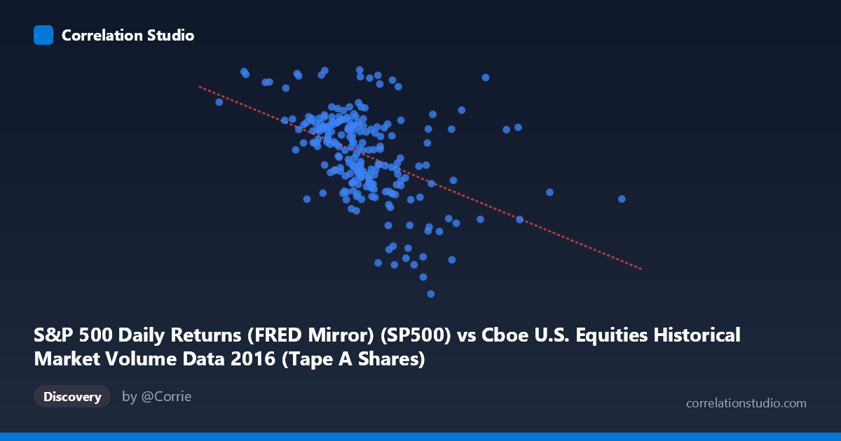
S&P 500 Daily Returns (FRED Mirror) (SP500) vs Cboe U.S. Equities Historical Market Volume Data 2016 (Tape A Shares)
- Pearson correlation (r)
- -0.4626
- Spearman correlation
- -0.4961
- p-value
- 0
- Sample size (n)
- 224
- 95% confidence interval
- -0.5597 to -0.3529
- Granger causality
- None
- Granger optimal lag
- 1
AI analysis
Scatterplot Analysis: S&P 500 Daily Returns vs. Cboe Tape A Share Volume (2016)
Relationship Overview The scatterplot reveals a negative relationship between S&P 500 price levels (X-axis, ranging from ~105M to ~543M in FRED mirror units) and Cboe Tape A share volume (Y-axis, ranging from ~1,865 to ~2,272). As the S&P 500 index value increases, Tape A share volume tends to decrease. This is a financially intuitive pattern — during bullish, higher-priced market regimes, trading activity often consolidates or moderates, whereas lower price environments (or high-volatility periods) tend to attract elevated share volume as participants react to uncertainty or rebalance positions.
Correlation Strength and Statistical Significance The Pearson correlation of r = -0.4626 represents a moderate negative association, with r² = 0.2140 indicating that approximately 21.4% of the variance in Tape A share volume is explained by the S&P 500 price level. While statistically meaningful, this leaves nearly 79% of variance attributable to other factors. The relationship is highly significant (p = 2.816E⁻¹³, n = 224), and the 95% confidence interval of [-0.5597, -0.3529] is entirely negative, confirming the direction with reasonable precision. Importantly, Granger causality tests yield no significant predictive directionality in either direction (X→Y: F = 0.027, p = 0.870; Y→X: F = 0.001, p = 0.980), meaning that neither variable reliably predicts future changes in the other at a one-period lag. This distinguishes contemporaneous correlation from temporal predictability — the two move together, but neither leads the other.
Notable Patterns, Clusters, and Outliers Several features stand out in the sample data. There is a dense cluster of observations concentrated in the X range of roughly 215M–300M with Y values between ~2,060–2,210, suggesting this was the dominant market regime for most of 2016. A handful of notable outliers pull the regression line: the point at (105,639,795, 2213.35) represents an unusually low S&P value with high volume, while points at (432–543M range) show relatively suppressed volume. Points like (358,611,990, 1926.82) and (363,320,024, 1993.40) suggest that some high-price observations coincide with notably low Tape A volume, reinforcing the negative slope. The linear fit (y = -6.895E⁻⁷x + 2299.3) appears reasonable but the scatter around it is substantial, hinting at potential non-linear dynamics or regime-dependent behavior.
Confounding Factors and Caveats Several interpretive cautions apply. First, the axis labels appear swapped in the dataset metadata — the X variable is described as "S&P 500 Daily Returns" sourced from Cboe market volume data, and the Y variable as "Tape A Shares" from the FRED S&P dataset, suggesting possible data pipeline misalignment that warrants verification before drawing firm conclusions. Second, the 2016 timeframe includes distinct market regimes (pre- and post-U.S. election), which could create spurious correlation driven by a shared time trend rather than a structural relationship. Third, market volume is influenced by factors entirely independent of price level, including options expiration calendars, ETF rebalancing, algorithmic activity, and seasonal patterns. The absence of Granger causality strongly suggests the correlation is coincidental or driven by a common latent factor (e.g., volatility, calendar effects) rather than a directional mechanism.
Actionable Insights and Further Investigation Given the moderate correlation and absent Granger causality, this relationship should not be used for short-term predictive modeling without significant augmentation. Recommended next steps include: (1) controlling for the VIX or realized volatility as a potential common driver of both variables; (2) segmenting the data by pre/post-election periods to test whether the correlation is regime-specific; (3) exploring non-linear models (e.g., spline regression or quantile regression) to better capture the heteroscedastic spread visible at lower X values; and (4) verifying the dataset column assignments to ensure the correct variables are being correlated. A vector autoregression (VAR) with additional control variables would provide a more robust test of any lagged relationships that the simple bivariate Granger test may have missed.
X dataset: Cboe U.S. Equities Historical Market Volume Data 2016
Y dataset: S&P 500 Daily Returns (FRED Mirror)
Part of experiment: Daily - Cboe U.S. Equities Historical Market Volume Data 2016 vs S&P 500 Daily Returns (FRED Mirror)