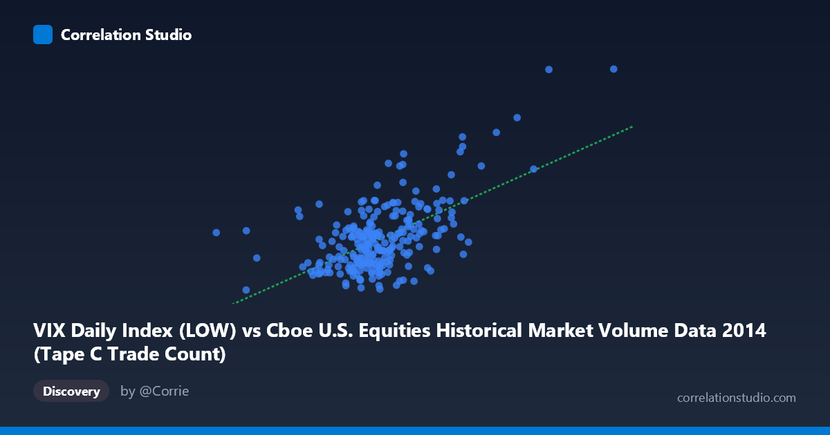
VIX Daily Index (LOW) vs Cboe U.S. Equities Historical Market Volume Data 2014 (Tape C Trade Count)
- Pearson correlation (r)
- 0.5945
- Spearman correlation
- 0.4526
- p-value
- 0
- Sample size (n)
- 252
- 95% confidence interval
- 0.5082 to 0.6689
- Granger causality
- None
- Granger optimal lag
- 1
AI analysis
Scatterplot Analysis: VIX Low vs. Tape C Trade Count (2014)
Relationship Overview
The scatterplot reveals a moderate positive relationship between the VIX Daily Index Low values and the Cboe U.S. Equities Tape C Trade Count across the 2014 trading year. As the VIX low rises — indicating elevated baseline fear or uncertainty in equity markets — the number of trades on Tape C (NYSE-listed securities reported to the consolidated tape) tends to increase correspondingly. This is intuitively consistent with market microstructure theory: periods of heightened volatility typically drive higher trading activity as market participants reposition, hedge, or react to uncertainty. The linear regression equation (y = 1.2437E-05x + 5.531) quantifies this relationship, suggesting that each unit increase in the VIX low is associated with a meaningful incremental rise in trade count, anchored from a baseline of approximately 5.53 million trades.
Correlation Strength and Statistical Significance
The Pearson correlation of r = 0.5945 indicates a moderate-to-strong positive association, but the more important figure for practical interpretation is r² = 0.3534 — meaning roughly 35.3% of the variance in Tape C trade counts is statistically explained by variation in the VIX low. While statistically robust (p ≈ 0, n = 252, N = 3,686), this also means ~65% of the variance remains unexplained by this variable alone, underscoring that VIX low is one of several meaningful drivers. The 95% confidence interval of [0.508, 0.669] is reassuringly tight and does not approach zero, lending high confidence that the true population correlation is meaningfully positive rather than a sampling artifact. Crucially, the Granger causality results are non-significant in both directions (X→Y: F = 2.38, p = 0.124; Y→X: F = 0.02, p = 0.883), meaning that neither variable reliably predicts the future values of the other at a 1-period lag. This is a critical caveat: the correlation is contemporaneous and associative, not predictive or directional in a temporal sense.
Notable Patterns, Clusters, and Outliers
The sample points reveal a broadly dispersed cloud with a discernible upward trend, but with considerable scatter at moderate X values (roughly 550,000–750,000), where trade counts range widely from ~10 to ~16. Several notable outliers stand out in the upper-right region of the plot: the point near (1,041,591, 24.61) is a clear extreme outlier, with both the highest VIX low and highest trade count in the sample, likely corresponding to a specific volatility event (e.g., geopolitical shock or macro data release) in 2014. Similarly, (841,278, 19.60) and (844,812, 16.08) form a secondary high-volume cluster. At the lower end, points like (728,415, 10.85) and (649,112, 10.34) suggest that high market volume does not always coincide with elevated VIX, indicating days of high-volume but low-fear trading. The distribution is not purely linear — there appear to be heteroscedastic tendencies, where variance in Y increases at higher X values, potentially limiting the reliability of a simple linear model.
Confounding Factors and Interpretive Caveats
Several confounding factors complicate a clean causal interpretation. First, day-of-week and seasonal effects in both equity volume and VIX are well-documented and could create spurious correlations. Second, Tape C specifically captures NYSE-listed stocks, so broader market events (e.g., S&P 500 index rebalancing, ETF arbitrage, option expiration dates) could simultaneously drive both variables upward without one causing the other. Third, the VIX "low" for a given day reflects intraday sentiment floors, which may be a less representative measure of daily volatility than the close or high. Fourth, the axes may be swapped from conventional expectation — the dataset labels suggest trade count is on the Y-axis but is drawn from the "VIX Daily Index" dataset, which warrants data provenance verification before drawing firm conclusions. Finally, macro-regime shifts within 2014 (e.g., Fed tapering completion, mid-year geopolitical events) could create structural breaks that the linear model ignores.
Actionable Insights and Further Investigation
Despite the non-significant Granger results, this correlation has practical relevance for trading operations, liquidity forecasting, and risk management. A VIX-informed trade volume model could help exchanges and market makers anticipate order flow surges, enabling better infrastructure scaling and spread management. To strengthen this analysis, several next steps are warranted: (1) test non-linear models (e.g., log-log or polynomial regression) given the apparent heteroscedasticity; (2) incorporate additional VIX metrics (close, high, daily range) alongside the low to build a multivariate predictor; (3) extend the time series beyond 2014 to test whether this r ≈ 0.59 relationship is stable across different volatility regimes; (4) apply rolling-window Granger causality tests to detect whether lead-lag relationships emerge during specific market stress periods; and (5) disaggregate by market sub-periods (e.g., pre- and post-October 2014 volatility spike) to identify whether the outlier cluster is regime-specific or broadly representative.
X dataset: Cboe U.S. Equities Historical Market Volume Data 2014
Y dataset: VIX Daily Index
Part of experiment: Daily - Cboe U.S. Equities Historical Market Volume Data 2014 vs VIX Daily Index