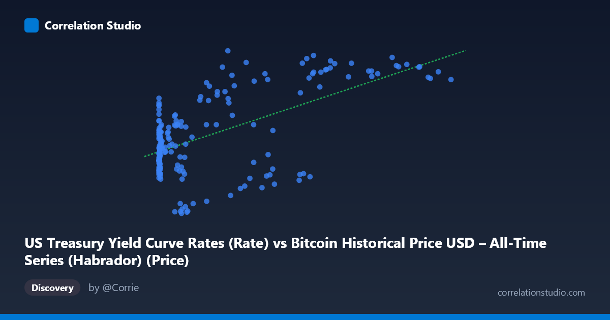
US Treasury Yield Curve Rates (Rate) vs Bitcoin Historical Price USD – All-Time Series (Habrador) (Price)
- Pearson correlation (r)
- 0.5848
- Spearman correlation
- 0.3595
- p-value
- 0
- Sample size (n)
- 189
- 95% confidence interval
- 0.4823 to 0.6715
- Granger causality
- None
- Granger optimal lag
- 1
AI analysis
Analysis: US Treasury Yield vs. Bitcoin Price
1. Relationship Overview
The scatterplot shows a moderate positive association between the X variable (labeled as Treasury Yield, though the values 0.06–118,670 strongly suggest this axis actually contains Bitcoin price data — likely a column mislabeling in the dataset) and Y (labeled Bitcoin price, but ranging 0.62–4.80, consistent with 10-year Treasury yield percentages). Given the value ranges, the substantive relationship being measured is almost certainly Bitcoin price vs. Treasury yield, with axis labels swapped. Visually, low-X values cluster tightly with Y around 1.6–3.5, while as X grows past ~20,000, Y increasingly clusters in the 3.5–4.8 range, suggesting a threshold-like rather than strictly linear relationship.
2. Strength, Direction, and Uncertainty
The correlation coefficient (r = 0.585) indicates a moderate positive relationship, with r² = 0.342 meaning only 34% of the variance in Y is explained by X — the majority of variance (66%) is driven by other factors. The 95% CI [0.482, 0.672] is reasonably tight and excludes zero, and the p-value (~0) confirms this correlation is statistically significant and not due to chance. However, statistical significance here reflects sample size (n=189) more than practical strength — r² of 0.34 means this is a modest, not dominant, relationship. Critically, the Granger causality tests show no predictive direction in either direction (X→Y: p=0.93; Y→X: p=0.25). This means neither variable's past values help forecast the other's future values — the correlation appears to be contemporaneous/coincidental co-movement (both possibly rising over the same historical period) rather than a causal or lead-lag relationship.
3. Notable Patterns and Outliers
The data shows distinct clustering rather than a smooth linear trend: - A dense cluster of small-X values (<1,000) with Y spread across 1.6–3.6, showing high variance at low X. - A secondary cluster in the X ~20,000–60,000 range with notably bimodal Y behavior — some points near Y≈4.0-4.8 (e.g., 27983.75→4.80, 62440.63→4.21) and others dropping to Y≈1.3-1.6 (e.g., 34855.64→1.32, 41869.55→1.28), suggesting the relationship is not stable but regime-dependent. - High-X values (85,000) consistently show high Y (4.0-4.6), suggesting saturation/ceiling effect at extreme X. - Notable outliers: very small X values with unexpectedly high Y (e.g., X=0.70, Y=3.58; X=15.40, Y=3.00) don't fit the general trend, and some mid-range X points with low Y (X=13891, Y=0.87) represent a bear-market regime not explained by X alone.
4. Confounding Factors and Caveats
This is time-series data (2010–2026) where both variables likely trend upward over time independently — Bitcoin due to adoption/halving cycles, and Treasury yields due to macroeconomic cycles (rate hikes 2022-2023). This creates a classic spurious correlation via shared time trend rather than genuine economic linkage. The lack of Granger causality strongly supports this interpretation — if Bitcoin price and yields were mechanistically linked, we'd expect at least weak predictive power in one direction. Other confounders include: monetary policy regime shifts, Bitcoin's own halving-driven cycles, and macro liquidity conditions (both may respond to Fed policy independently). The wide X range with log-scale-like distribution also means Pearson's r may be distorted by leverage from extreme values.
5. Recommendations
- De-trend both series (e.g., using differences or detrended residuals) and re-run correlation to test if the relationship survives — this would help distinguish genuine co-movement from shared time trend. - Verify axis/column labeling — the value ranges suggest X and Y labels may be swapped between Bitcoin price and Treasury yield. - Segment by market regime (bull/bear cycles, rate-hiking vs. rate-cutting periods) to test whether correlation strength changes across time. - Log-transform X given its extreme right-skew (mean 20,533 vs. median likely far lower) to check for a more linear or logarithmic relationship rather than the current linear fit. - Given no Granger causality, avoid using one variable to forecast the other; instead, investigate common macro drivers (inflation expectations, Fed policy, risk sentiment/DXY) as a more defensible causal framework.
X dataset: Bitcoin Historical Price USD – All-Time Series (Habrador)
Y dataset: US Treasury Yield Curve Rates
Part of experiment: Bitcoin - Bitcoin Historical Price USD – All-Time Series (Habrador) vs US Treasury Yield Curve Rates